2 Univariate Hawkes

A univariate Hawkes process (Hawkes (1971)) is defined to be a self-exciting temporal point process where the conditional intensity function is given by

\[\lambda(t) = \mu(t) + \Sigma_{i:\tau_i<t}\nu(t-\tau_i).\]

Here $\mu(t)$ is the background rate of the process and $\Sigma_{i:\tau_i<t}\nu(t-\tau_i)$ is some historic temporal dependence (i.e., for times $\tau_i < t$, $ i = 1, …, T$). The classic homogeneous formulation uses an exponential decay kernal:

\[\lambda(t) = \mu + \alpha \Sigma_{i:\tau_i<t}\text{exp}(-\beta * (t-\tau_i)). \tag{2.1}\]

Here the parameter $\alpha$ is the increase in intensity immediately after the occurrence of an event, and $\beta > 0$ controls the exponential decay of the intensity if no event has occurred. To avoid the conditional intensity heading off to infinity $\beta > \alpha$. See (hawkesnll?) for the negative log-likelihood written in R syntax.

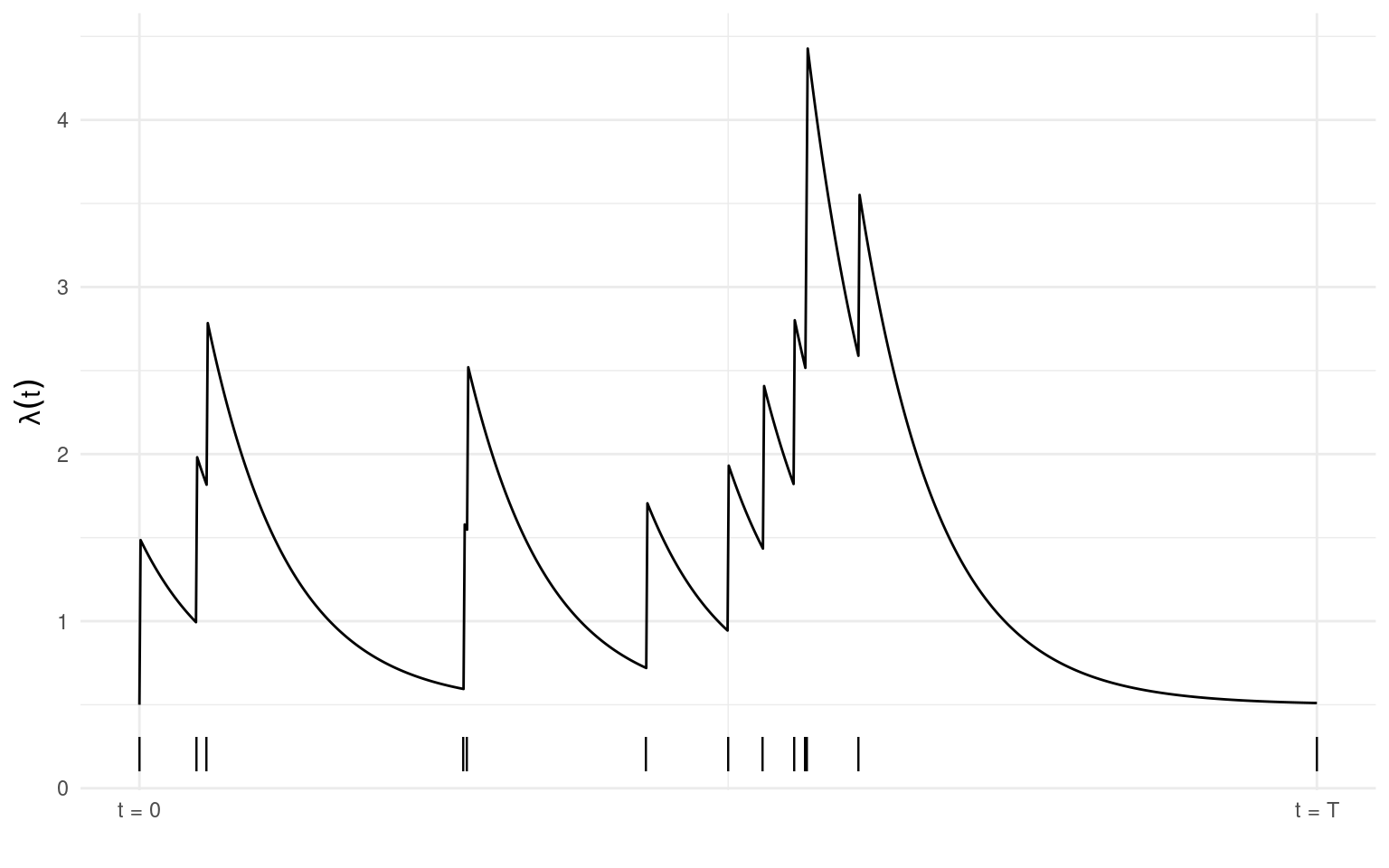
Plotted below is the conditional intensity ($\lambda(t), t \in [0,T]$) of a Hawkes process with $\mu = 0.1$, $\alpha = 1$, and $\beta = 1.5$. Observed events (n = 13) are shown by the vertical dashes along the x-axis. The intensity increases immediately after an event occurs and decays exponentially over time if no event is observed for some period.

2.1 Simulating from a univariate Hawkes model

The function sim_hawkes() offers two simulation methods for simulating a realisation of a univariate Hawkes process. The default, with method = 1, uses the same method as algorithm 2 in Ogata (1981), simulating until a given time horizon (set by argument n).

sim <- sim_hawkes(mu = 0.5, alpha = 1, beta = 1.5, n = 40, plot = TRUE)

The second option, setting method = 2, uses an accept/reject framework and the argument n specifies the number of points to simulate (default n = 100).

sim <- sim_hawkes(mu = 0.5, alpha = 1, beta = 1.5, plot = TRUE, method = 2)

2.2 Fitting a univariate Hawkes model

require(stelfi)

To fit a univariate Hawkes model in stelfi use the function fit_hawkes() with the following required arguments

times - a vector of numeric occurrence times, and
parameters - a vector of named starting values for $\mu$ (mu), $\alpha$ (alpha), and $\beta$ (beta).

The function get_coefs() can then be called on the fitted model object to return the estimated parameter values.

2.2.1 A simulated example

Simulating a realisation of a univariate Hawkes process (see Section 2.1 for more details) with $\mu = 1.3$, $\alpha = 0.4$, and $\beta = 1.5$ (over $t \in [0, 500]$).

times <- sim_hawkes(mu = 1.3, alpha = 0.4, beta = 1.5, n = 500)

## starting values
sv <- c(mu = 1.3, alpha = 0.4, beta = 1.5)
## using stelfi
fit <- fit_hawkes(times = times, parameters = sv)
stelfi <- get_coefs(fit)
stelfi

       Estimate Std. Error
mu    1.3997320  0.1125668
alpha 0.3737118  0.1207772
beta  1.7730216  0.7495558

As a comparison, below emhawkes (Lee (2023)), and hawkesbow (Cheysson (2021)) are used to fit a univariate Hawkes process to the same simulated data.

## benchmark using emhawkes
require(emhawkes)
h <- new("hspec", mu = sv[1], alpha = sv[2], beta = sv[3])
## emhawkes requires the inter arrival times to fit the model
inter <- diff(times)
fit_em <- hfit(object = h, inter_arrival = inter)
em <- summary(fit_em)$estimate
em

        Estimate Std. error   t value      Pr(> t)
mu1    1.3976553  0.1091437 12.805644 1.524557e-37
alpha1 0.3683585  0.1380857  2.667608 7.639335e-03
beta1  1.7380101  0.8236957  2.110015 3.485708e-02

## bench mark using hawkesbow
require(hawkesbow)
fit_bow <- mle(events = times, kern = "Exponential", end = max(times))
## use the Hessian to obtain the standard errors from hawkesbow
bow <- cbind(Estimate = fit_bow$par,
         "Std. error" = -fit_bow$model$ddloglik(times, max(times)) |> solve() |> diag() |> sqrt())
bow

      Estimate Std. error
[1,] 1.3998368 0.11238176
[2,] 0.2107781 0.05814911
[3,] 1.7724499 0.74877227

The table below gives the estimated parameter values from each of stelfi, emhawkes, and hawkesbow along with the standard errors in brackets. Note that hawkesbow estimates $\frac{\alpha}{\beta}$ rather that $\beta$ directly, and that the standard errors are computed here using the returned Hessian matrix $H$ (i.e., $\sqrt{\text{diag}{-(H^{-1})}}$).

	$\mu$	$\alpha$	$\beta$	$\frac{\alpha}{\beta}$
TRUTH	1.300	0.400	1.500	0.267
stelfi	1.4 ( 0.113 )	0.374 ( 0.121 )	1.773 ( 0.75 )	-
emhawkes	1.398 ( 0.109 )	0.368 ( 0.138 )	1.738 ( 0.824 )	-
hawkesbow	1.4 ( 0.112 )	-	1.772 ( 0.749 )	0.211 ( 0.058 )

2.2.2 An applied example

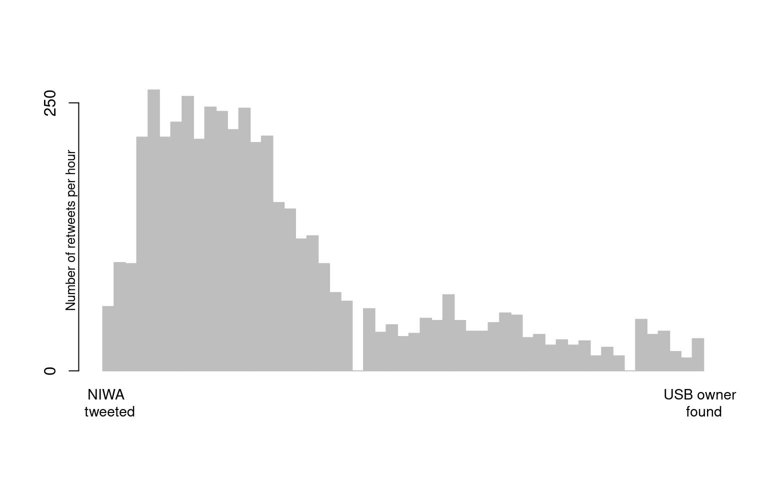
A NIWA scientist found a working USB in the scat of a leopard seal, they then tweeted about it in the hopes of finding its owner¹. The dates and times of these tweets and retweets are available in stelfi as retweets_niwa.

data(retweets_niwa)

The dates/times need to be numeric and sorted in ascending order (starting a time $t = 0$). Note too that there can be no simultaneous events.

## numeric time stamps
times <- unique(sort(as.numeric(difftime(retweets_niwa ,min(retweets_niwa),units = "mins"))))

The histogram below shows the observed counts (4772) of unique retweet times from the original tweet ($t=0$) to the time (just over two days later) that the owner of the USB came forward, t = 3143 mins.

To fit the model chose some starting values for the parameters and supply these along with the numeric times to the function fit_hawkes().

sv <- c(mu = 9, alpha = 3, beta = 10)
fit <- fit_hawkes(times = times, parameters = sv)

## print out estimated parameters
pars <- get_coefs(fit)
pars

        Estimate  Std. Error
mu    0.06328099 0.017783908
alpha 0.07596531 0.007777899
beta  0.07911346 0.008109789

From the estimated coefficients above

the expected (estimated) background rate of sightings (i.e., independent sightings) is $\hat{\mu}T =$ 0.063 $\times$ 3143.02 $=$ 198.89, which indicates that ~199 retweets (from the 4772) were principal retweets and that the remaining were due to self-excitement;
the expected number of retweets “triggered” by any one retweet is estimated as $\frac{\hat{\alpha}}{\hat{\beta}}$ = 0.96 (note the maximum this can possibly be is 1);
the expected number of descendants per retweet is estimated as $\frac{\hat{\beta}}{\hat{\beta} - \hat{\alpha}}$ = 25.13;
the rate of decay for the self-excitement is estimated as $\frac{1}{\hat{\beta}}$ = 12.64, indicating that after ~13 minutes a retweet is likely unrelated² to the previous retweet.

The show_hawkes() function can be called on the fitted model object to plot the estimated conditional intensity and the data, top and bottom panels below respectively.

show_hawkes(fit)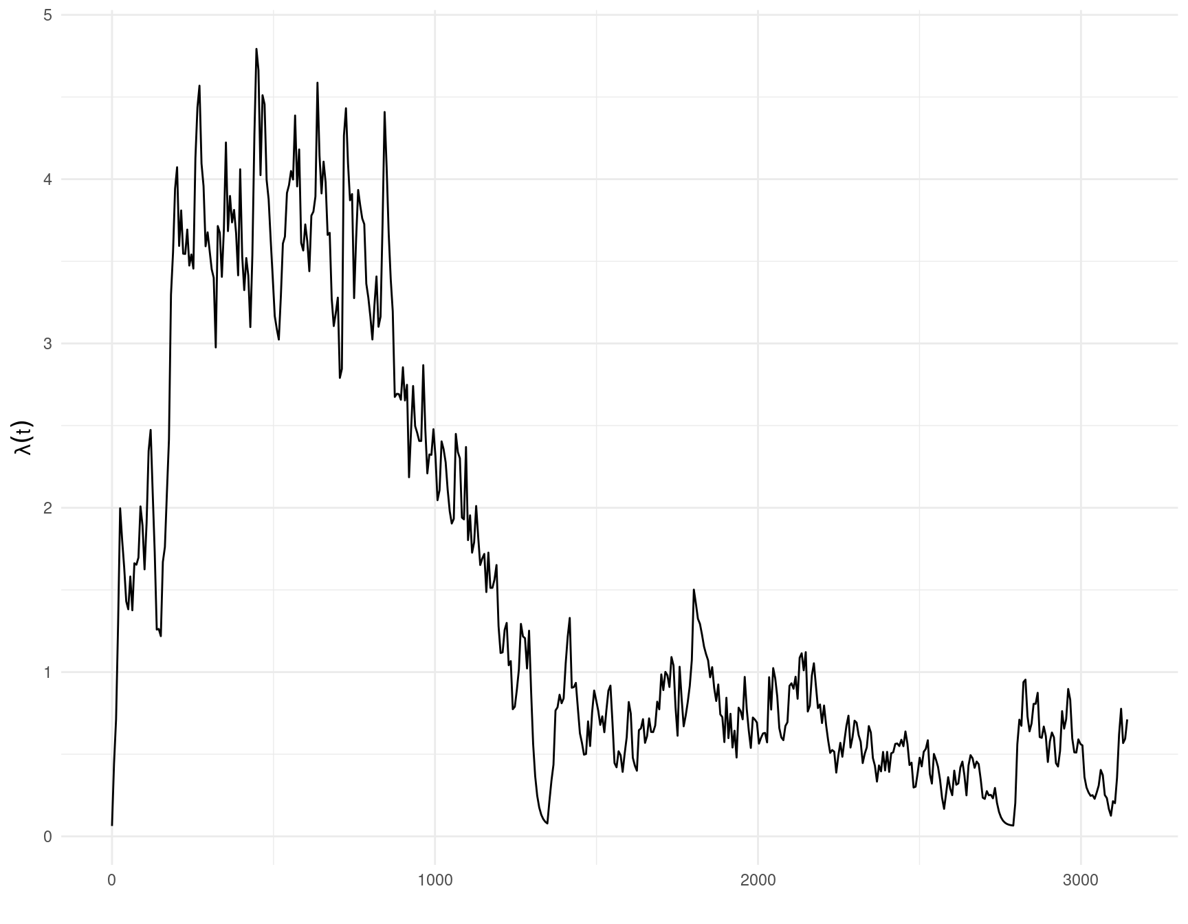

2.3 Goodness-of-fit for a univariate Hawkes process

The compensator, $\Lambda(\tilde{t})$, of any inhomogeneous Poisson process gives the expected number of events in some defined interval $[0, \tilde{t}]$ is given by

\[\Lambda(\tilde{t}) = \int_0^{\tilde{t}} \lambda(t) dt.\]

The random change theorem (Daley, Vere-Jones, et al. (2003)) states that if a set of events $[\tau_1, ..., \tau_n]$ is a realisation from a inhomogeneous Poisson process then $[\Lambda(\tau_1), ..., \Lambda(\tau_n)]$ is a realisation of a homogeneous Poisson process with unit rate. Letting $\delta \Lambda_{i} = \Lambda(\tau_i) - \Lambda(\tau_{i-1})$ for $i = 2, ..., N$ and $\delta \Lambda_{1} = \Lambda(\tau_1)$, under the theorem above $\delta \Lambda_{i} \sim \text{Exp}(1)$. Using this result a typical goodness-of-fit test is a Kolmogorov-Smirnov (KS) test (see Daley, Vere-Jones, et al. (2003) for more details) where the KS statistic is a measure of the distance between the empirical distribution of all $\delta \Lambda_{i}$ and the CDF of a $\text{Exp}(1)$ distribution.

The compensator differences can be extracted from a fitted model using the compensator_differences() function, and a KS test can be carried out manually:

times <- sim_hawkes(mu = 1.3, alpha = 0.4, beta = 1.5, n = 500)
sv <- c(mu = 2, alpha = 1, beta = 5)
fit <- fit_hawkes(times = times, parameters = sv)
compensator <- compensator_differences(fit)
stats::ks.test(compensator, "pexp")


    Asymptotic one-sample Kolmogorov-Smirnov test

data:  compensator
D = 0.013855, p-value = 0.9958
alternative hypothesis: two-sided

This gives no evidence against the compensator values coming from a $\text{Exp}(1)$ distribution.

Another goodness-of-fit test is the Box-Ljung (or Ljung–Box) test, which tests for autocorrelation between the consecutive compensator values (i.e., independence/stationarity).

stats::Box.test(compensator, type = "Ljung")


    Box-Ljung test

data:  compensator
X-squared = 0.66599, df = 1, p-value = 0.4145

This gives no evidence against the consecutive compensator values being independently distributed.

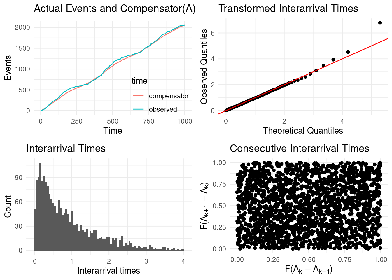
Alternatively, both tests and some diagnostic plots are returned by calling the show_hawkes_GOF() function. The four panels an be interpreted as follows

top left, plots the compensator values against the observed times, which under a well fitting model should align;
top right, a transformed QQ plot, the observed quantities should align with the theoretical quantiles under a well fitting model;
bottom left, the compensator differences, which under the model are assumed to be $\text{Exp}(1)$ distributed;
bottom right, consecutive compensator differences, which should show no obvious pattern (no autocorrelation evident) under a well fitting model.

show_hawkes_GOF(fit)


    Asymptotic one-sample Kolmogorov-Smirnov test

data:  interarrivals
D = 0.013855, p-value = 0.9958
alternative hypothesis: two-sided


    Box-Ljung test

data:  interarrivals
X-squared = 0.66599, df = 1, p-value = 0.4145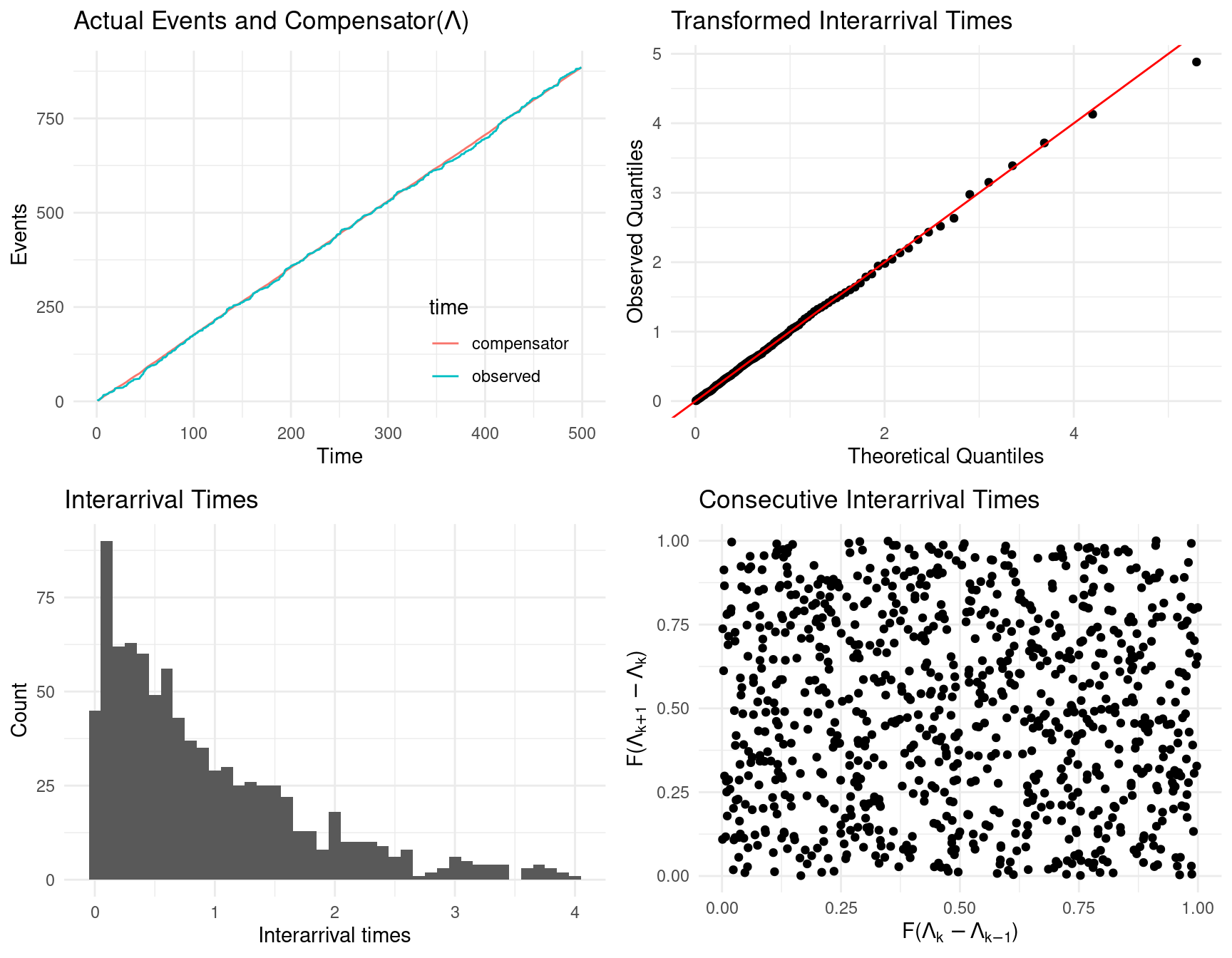

2.4 Fitting an inhomogenous Hawkes model

A univariate inhomogenous Hawkes process has $\mu = \mu(t)$ in Equation 2.1 (i.e., the baseline is time varying, rather than being constant).

Below we simulate data from a Hawkes process with $\mu(t) = [A + B*\text{sin}(\frac{2 \pi t}{365.25})]$ (with $A = 1$ and $B = 0.5$) to represent a yearly cycle and self-exciting parameters $\alpha = 1$ and $\beta = 2$ using hawkesbow (Cheysson (2021)).

mut <- function(t) {
 1 + 0.5*sin((2*pi*t)/365.25)
}

set.seed(1)
times <- hawkesbow::hawkes(1000, fun = mut,
 M = 1.5, repr = 0.5, family = "exp", rate = 2)$p

To fit this model in stelfi the function $\mu(t)$ (background) and its integral $\int_0^t \mu(y) dy$ (background_integral) are supplied by the user. To ensure $\mu(t) > 0$ below $\mu(t)$ is written as a function of $x$ and $y$, where $A = e^x$ and $B = \text{logit}(y) e^x$.

background <- function(params,t){
        A = exp(params[[1]])
        B = stats::plogis(params[[2]]) * A
        return(A + B*sin((2*pi*t)/365.25))
}

background_integral <- function(params,x){
        A = exp(params[[1]])
        B = stats::plogis(params[[2]]) * A
        return((A*x)-B*cos((2*pi*x)/365.25))
}

These functions are then passed to the function fit_hawkes_cbf() alongside the observed times (times) and a list of starting values for both $\mu(t)$ and the self-exciting components via the argument background_parameters and parameters respectively.

sv = list(alpha = 0.5, beta = 1.5)
background_sv = list(1,1)
fit <- fit_hawkes_cbf(times = times, parameters = sv,
background = background, background_integral = background_integral, background_parameters = background_sv)

The estimated values of the the transformed $A$ and $B$ parameters are returned via fit$background_parameters, the code below transforms them back to the original scale.

exp(fit$background_parameters[1])

[1] 1.135523

plogis(fit$background_parameters[2]) * exp(fit$background_parameters[1])

[1] 0.7755937

The estimated values of the self-excitement parameters $\alpha$ and $\beta$ are returned by the get_coefs() function as usual. The table below compares the estimated values to the true ones

	$A$	$B$	$\alpha$	$\beta$
TRUTH	1.000	0.500	1.000	2.000
stelfi	1.136	0.776	0.985	2.198

The function show_hawkes() can be used to show the fitted model.

show_hawkes(fit)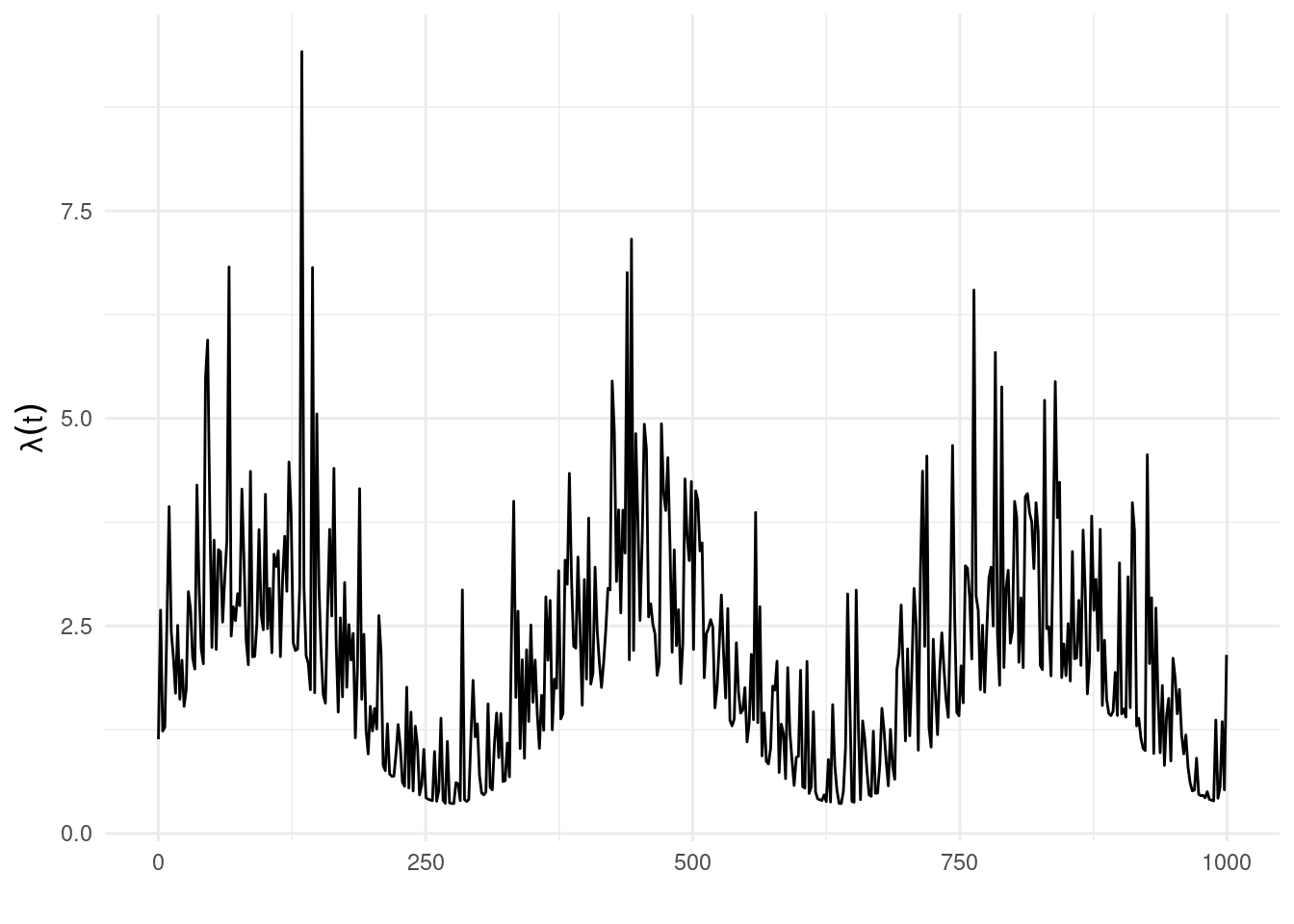

The function show_hawkes_GOF() will show/print the model diagnostics discussed in Section 2.3.

show_hawkes_GOF(fit)


    Asymptotic one-sample Kolmogorov-Smirnov test

data:  interarrivals
D = 0.018277, p-value = 0.4985
alternative hypothesis: two-sided


    Box-Ljung test

data:  interarrivals
X-squared = 28.608, df = 1, p-value = 8.86e-08

This was at the time it was called Twitter (not X) so ‘tweet’ is the correct term!↩︎
Note that unrelated is not quite the correct term here, rather that the event is likely a baseline event rather than due to self-excitement↩︎