5  Spatial log-Gaussian Cox process

A log-Gaussian Cox Process (LGCP) is a doubly stochastic spatial point process. In the simplest case, the intensity of the point process over space is given by \[\Lambda(s) = \text{exp}(\beta_0 + G(s) + \epsilon)\] where \(\beta_0\) is a constant, known as the intercept, \(G(s)\) is a Gaussian Markov Random Field (GMRF) and \(\epsilon\) an error term.

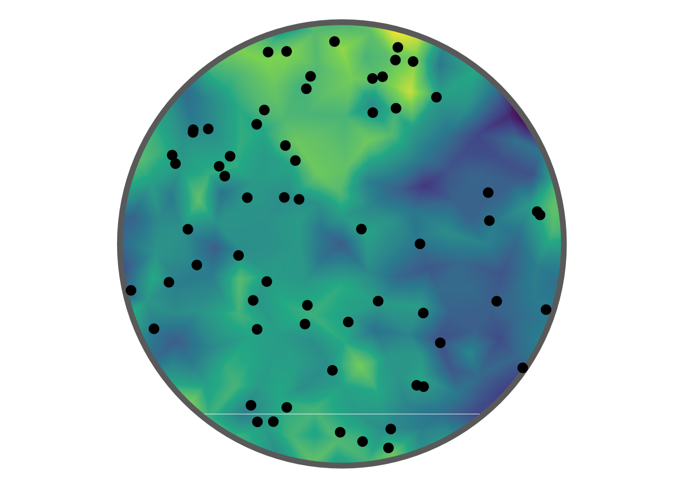
Plotted below is a realisation of a LGCP within a disc shaped region overlain on the latent GMRF.

Following the Stochastic Partial Differential Equation (SPDE) approach proposed by Lindgren, Rue, and Lindström (2011) a Matérn covariance function is assumed for \(G(s)\):

\[C(r; \sigma, \kappa) = \frac{\sigma^2}{2^{\nu-1} \Gamma(\nu)} (\kappa \:r)^\nu K_\nu(\kappa \: r)\]

where \(\kappa\) is a scaling parameter and \(\sigma^2\) is the marginal variance (\(\nu\) is typically fixed, see Lindgren, Rue, and Lindström (2011)). Rather than the scaling parameter, a range parameter \(r=\frac{\sqrt{8}}{\kappa}\) is typically interpreted (corresponding to correlations near 0.1 at the distance \(r\)). The standard deviation is given as \(\sigma=\frac{1}{\sqrt{4\pi\kappa^2\tau^2}}\). In the figure above \(\beta = 3\), \(\text{log}(\tau) = 1.6\), and \(\text{log}(\kappa) = 1.95\).

5.1 Delauney triangluations when fitting LGCP models

TODO

5.2 Fitting a LGCP model

Using spatstat to simulate a LGCP

win <- spatstat.geom::disc()
## here mu is beta0
set.seed(1234)
sim <- spatstat.random::rLGCP("matern", mu = 3,
               var = 0.5, scale = 0.7, nu = 1,
               win = win)

## plotting the simulated (log) random field using ggplot
xs = attr(sim, "Lambda")$xcol; ys = attr(sim, "Lambda")$yrow
pxl <- expand.grid(x = xs, y = ys)
pxl$rf <- as.vector(attr(sim, "Lambda")$v) |> log() - 3 ## minus the intercept
require(ggplot2)
ggplot() + 
  geom_tile(data = pxl, aes(x = x, y = y, fill = rf), )  +
  labs(fill = "") + xlab("") + ylab("") + 
  scale_fill_viridis_c(option = "D", na.value = NA) +
  coord_equal() + theme_void() +
  geom_sf(data = sf::st_as_sf(win), fill = NA, linewidth = 2) +
  geom_point(data = data.frame(x = sim$x, y = sim$y), aes(x = x, y = y))

Fitting a model using stelfi

## dataframe of point locations 
locs <- data.frame(x = sim$x, y = sim$y)
## Delauney triangulation of domain
smesh <- fmesher::fm_mesh_2d(loc = locs[, 1:2], max.edge = 0.2, cutoff = 0.1)
## sf of domain
sf <- sf::st_as_sf(win)
fit <- fit_lgcp(locs = locs, sf = sf, smesh = smesh,
                parameters = c(beta = 3, log_tau = log(1),
                               log_kappa = log(1)))
get_coefs(fit)                 

            Estimate Std. Error
beta       3.2180075  0.2678925
log_tau   -1.9447694  0.7069575
log_kappa  1.3917981  0.5967719
range      0.7032258  0.4196654
stdev      0.4903966  0.1469378

The estimated GMRF can be plotted using the show_field() function once the values have been extracted using get_fields().

get_fields(fit, smesh) |>
    show_field(smesh = smesh, sf = sf, clip = TRUE) + theme_void() +
    geom_point(data = data.frame(x = sim$x, y = sim$y), aes(x = x, y = y))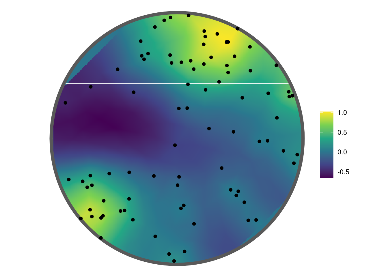

As a comparison, inlabru (Bachl et al. (2019)) is used to fit the same model to these data.

require(inlabru)
require(sp)
locs_sp <- locs; sp::coordinates(locs_sp) <- c("x", "y")
domain <- as(sf, "Spatial")
matern <- INLA::inla.spde2.pcmatern(smesh, prior.sigma = c(0.7, 0.01), prior.range = c(4, 0.5) )
## latent field
cmp <- coordinates ~ random_field(coordinates, model = matern) + Intercept(1)
sp::proj4string(locs_sp) <- smesh$crs <- sp::proj4string(domain)
## fit model
fit_inla <- lgcp(cmp, locs_sp, samplers = domain, domain = list(coordinates = smesh))
pars <- rbind(fit_inla$summary.fixed[,1:2], fit_inla$summary.hyperpar[,1:2])
pars

                            mean        sd
Intercept              3.2755781 0.6680163
Range for random_field 1.7795900 0.9046165
Stdev for random_field 0.4655544 0.1621035

Now using spatstat

ss <- spatstat.model::lgcp.estK(sim, covmodel = list(model = "matern", nu = 1))
ss$clustpar

      var     scale 
0.3541098 0.3018202 

ss$modelpar

   sigma2     alpha        mu 
0.3541098 0.3018202 3.1445250 

The table below gives the estimated parameter values from stelfi and inlabru along with the standard errors in brackets (where possible).

	\(\beta_0\)	\(r\)	\(\sigma\)
stelfi	3.218 ( 0.268 )	0.703 ( 0.42 )	0.49 ( 0.147 )
inlabru	3.276 ( 0.668 )	1.78 ( 0.905 )	0.466 ( 0.162 )
spatstat	3.145	0.854	0.595

5.2.1 An applied example

Using the applied example given in Jones-Todd and van Helsdingen (2024) a LGCP model is fitted to sasquatch sightings using the function fit_lgcp(). For more details on the use of the Delauney triangulation see Section 5.1.

data("sasquatch", package = "stelfi")
## get sf of the contiguous US
sf::sf_use_s2(FALSE)
us <- maps::map("usa", fill = TRUE, plot = FALSE) |>
    sf::st_as_sf() |>
    sf::st_make_valid()
## dataframe of sighting locations (lat, long)
locs <- sf::st_coordinates(sasquatch) |>
   as.data.frame()
names(locs) <- c("x", "y")
## Delauney triangulation of domain
smesh <- fmesher::fm_mesh_2d(loc = locs[, 1:2], max.edge = 2, cutoff = 1)
## fit model with user-chosen parameter starting values
fit <- fit_lgcp(locs = locs, sf = us, smesh = smesh,
                parameters = c(beta = 0, log_tau = log(1),
                               log_kappa = log(1)))
get_coefs(fit)                 

            Estimate Std. Error
beta      -0.7659374  0.3558810
log_tau   -0.6109840  0.1028264
log_kappa -0.9540269  0.1510160
range      7.3430015  1.1089108
stdev      1.3491825  0.1480772

Again, the estimated GMRF can be plotted using the show_field() function once the values have been extracted using get_fields().

get_fields(fit, smesh) |>
    show_field(smesh = smesh, sf = us, clip = TRUE) + ggplot2::theme_classic()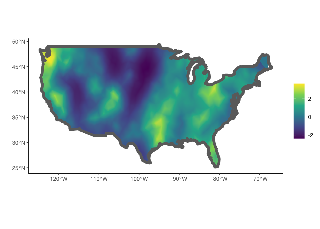

The estimated intensity surface can be plotted using the show_lambda() function.

show_lambda(fit, smesh = smesh, sf = us, clip = TRUE) + ggplot2::theme_classic()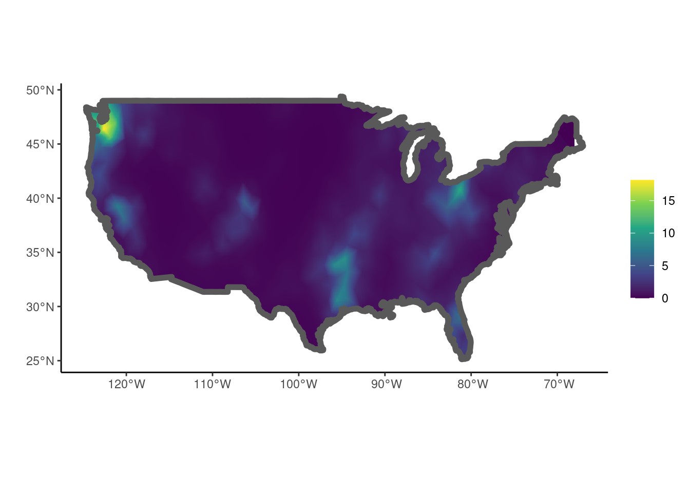

Again, as a comparison, inlabru (Bachl et al. (2019)) is used to fit the same model to these data.

require(inlabru)
require(sp)
locs_sp <- locs; sp::coordinates(locs_sp) <- c("x", "y")
domain <- as(us, "Spatial")
matern <- INLA::inla.spde2.pcmatern(smesh,
prior.sigma = c(0.1, 0.01),
prior.range = c(5, 0.01)
)
## latent field
cmp <- coordinates ~ random_field(coordinates, model = matern) + Intercept(1)
sp::proj4string(locs_sp) <- smesh$crs <- sp::proj4string(domain)
## fit model
fit_inla <- lgcp(cmp, locs_sp, samplers = domain, domain = list(coordinates = smesh))
pars <- rbind(fit_inla$summary.fixed[,1:2], fit_inla$summary.hyperpar[,1:2])
pars

                             mean         sd
Intercept              -0.4907638 0.24998054
Range for random_field  7.9401368 0.81253926
Stdev for random_field  0.8759888 0.06323398

The table below gives the estimated parameter values from stelfi and inlabru along with the standard errors in brackets.

	\(\beta_0\)	\(r\)	\(\sigma\)
stelfi	-0.766 ( 0.356 )	7.343 ( 1.109 )	1.349 ( 0.148 )
inlabru	-0.491 ( 0.25 )	7.94 ( 0.813 )	0.876 ( 0.063 )

5.3 SPDE as GAM

TODO

Bachl, Fabian E., Finn Lindgren, David L. Borchers, and Janine B. Illian. 2019. “inlabru: An R Package for Bayesian Spatial Modelling from Ecological Survey Data.” Methods in Ecology and Evolution 10: 760–66. https://doi.org/10.1111/2041-210X.13168.

Jones-Todd, Charlotte M., and Alec B. M. van Helsdingen. 2024. “stelfi: An R Package for Fitting Hawkes and Log-Gaussian Cox Point Process Models.” Ecology and Evolution 14: e11005. https://doi.org/10.1002/ece3.11005.

Lindgren, Finn, Håvard Rue, and Johan Lindström. 2011. “An Explicit Link Between Gaussian Fields and Gaussian Markov Random Fields: The Stochastic Partial Differential Equation Approach (with Discussion).” Journal of the Royal Statistical Society B 73 (4): 423–98.