data(package = "stelfi")$result[, "Item"] [1] "horse_mesh" "horse_sf" "iraq_terrorism" "marked"
[5] "multi_hawkes" "nz_earthquakes" "nz_murders" "retweets_niwa"
[9] "sasquatch" "uk_serial" "xyt" stelfiBelow are the data packaged within stelfi.
data(package = "stelfi")$result[, "Item"] [1] "horse_mesh" "horse_sf" "iraq_terrorism" "marked"
[5] "multi_hawkes" "nz_earthquakes" "nz_murders" "retweets_niwa"
[9] "sasquatch" "uk_serial" "xyt" ## load the tidyverse packages
library(tidyverse)retweets_niwaIn 2019 a NIWA scientist found a working USB in the scat of a leopard seal, they then tweeted about it in the hopes of finding its owner. In this chapter a Hawkes process is fitted to these data.
NIWA is searching for the owner of a USB stick found in the poo of a leopard seal…
— Earth Sciences New Zealand (@earthsciencesnz) February 5, 2019
Recognise this video? Scientists analysing the scat of leopard seals have come across an unexpected discovery – a USB stick full of photos & still in working order! https://t.co/2SZVkm5az4 pic.twitter.com/JLEC8vuHH0
The retweets_niwa dataset contains the retweet timestamps for this tweet.
data(retweets_niwa, package = "stelfi")
head(retweets_niwa)
[1] "2019-02-07 06:50:08 UTC" "2019-02-07 06:50:08 UTC"
[3] "2019-02-07 06:49:22 UTC" "2019-02-07 06:48:48 UTC"
[5] "2019-02-07 06:47:52 UTC" "2019-02-07 06:47:42 UTC"ggplot(data.frame(time = retweets_niwa), aes(x = time)) +
geom_histogram() + ylab("Retweet frequency") + xlab("") +
theme_bw()`stat_bin()` using `bins = 30`. Pick better value with `binwidth`.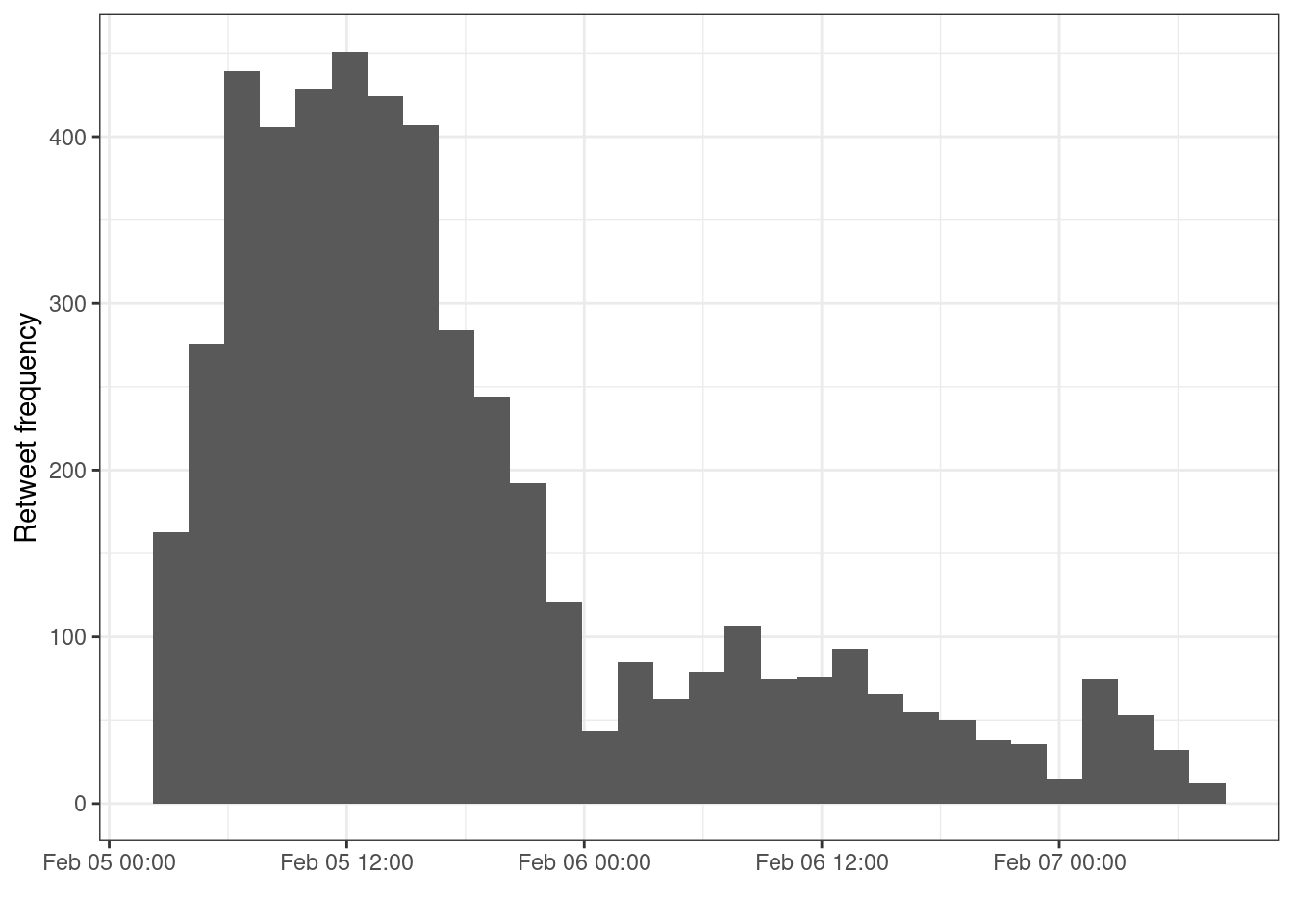
uk_serialMurder UK documents some of the UKs most infamous multiple murderer cases. The uk_serial dataset contains summary information about the documented cases along with approximate timeframes.
data("uk_serial", package = "stelfi")
head(uk_serial)
number_of_kills years name aka
1 300 1995 - 1998 Dr. Harold Shipman Dr. Death
2 160 1949 - 1983 Dr. John Bodkin Adams
3 26 1978 Peter Dinsdale Bruce Lee
4 21 1865 - 1872 Mary Ann Cotton
5 16 1828 William Burke and William Hare Body Snatchers
6 15 1944 - 1948 John George Haigh Acid Bath Murderer
year_start year_end date_of_first_kill population_million
1 1995 1998 03/1995 58.02
2 1949 1983 08/1949 50.32
3 1973 NA 06/1973 56.19
4 1865 1872 01/1865 24.36
5 1828 NA 02/1828 15.73
6 1944 1948 09/1944 49.02uk_serial %>%
mutate(time = paste(date_of_first_kill, "/01", sep='')) %>%
mutate(time = as.Date(time, "%m/%Y/%d")) %>%
ggplot(aes(x = time)) +
geom_histogram() +
ylab("Frequency of known first kill") +
xlab("") + theme_bw()`stat_bin()` using `bins = 30`. Pick better value with `binwidth`.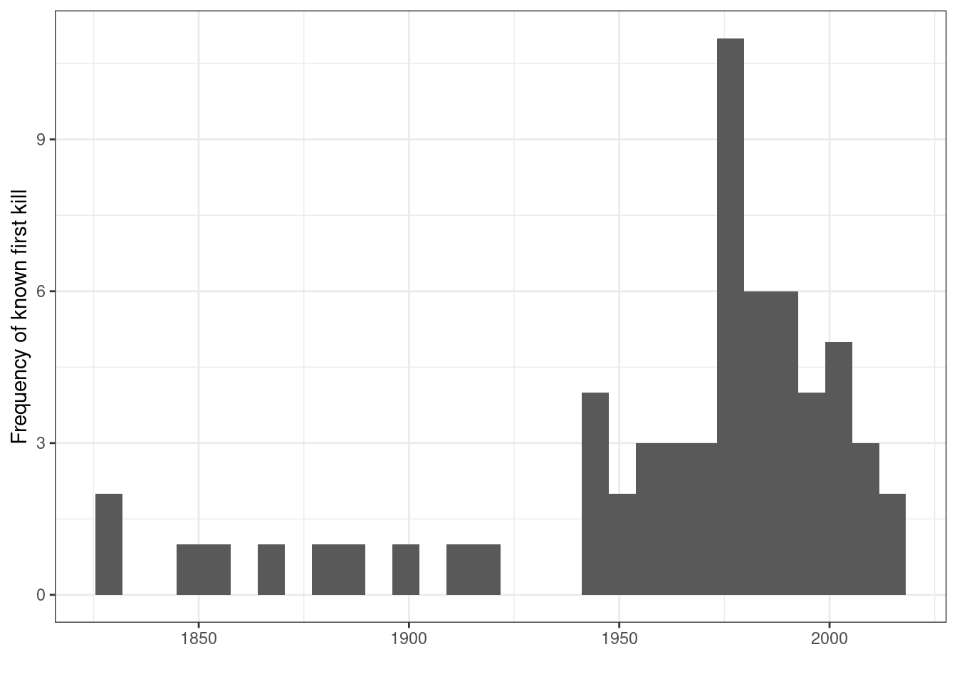
Using maps to create sf objects of country boundaries:
us <- maps::map("usa", fill = TRUE, plot = FALSE) %>%
    sf::st_as_sf() %>%
    sf::st_make_valid()
nz <- maps::map("nz", fill = TRUE, plot = FALSE) %>%
    sf::st_as_sf() %>%
    sf::st_make_valid()
iraq <- maps::map("world", "Iraq", fill = TRUE, plot = FALSE) %>%
     sf::st_as_sf() %>%
sf::st_make_valid()sasquatchThe Bigfoot Field Researchers Organization (BFRO) documents Bigfoot (Sasquatch) sightings; some data have been collated and packaged in stelfi assasquatch.
data("sasquatch", package = "stelfi")
sasquatch
Simple feature collection with 972 features and 27 fields
Geometry type: POINT
Dimension: XY
Bounding box: xmin: -124.5301 ymin: 25.84875 xmax: -70.75587 ymax: 48.9058
Geodetic CRS: +proj=longlat +datum=WGS84 +no_defs +ellps=WGS84 +towgs84=0,0,0
# A tibble: 972 × 28
observed location_details county state season title date number
* <chr> <chr> <chr> <chr> <chr> <chr> <date> <dbl>
1 "For the past f… This location i… Shann… Sout… Fall Repo… 2002-12-04 5173
2 "My family had … East on Route 1… Wayne… New … Fall Repo… 2003-09-20 26566
3 "While this inc… Ward County, Ju… Ward … Nort… Spring Repo… 2000-04-21 751
4 "(Please see Mi… <NA> Mount… Nort… Winter Repo… 2004-02-22 8165
5 "I was coming h… forested wetlan… Warre… New … Summer Repo… 2005-12-21 13276
6 "My summer ecol… We were on the … Taos … New … Spring Repo… 2000-05-17 4904
7 "On Aug 26 arou… From Garrison t… McLea… Nort… Summer Repo… 2005-08-27 12562
8 "Foot prints wh… The location wa… McKen… Nort… Winter Repo… 2004-02-26 8130
9 "The following … Georgia Ave. an… Sarpy… Nebr… Summer Repo… 2005-01-06 7809
10 "We live near O… (Location withh… Dougl… Nebr… Summer Repo… 2005-08-13 12482
# ℹ 962 more rows
# ℹ 20 more variables: classification <chr>, geohash <chr>,
# temperature_high <dbl>, temperature_mid <dbl>, temperature_low <dbl>,
# dew_point <dbl>, humidity <dbl>, cloud_cover <dbl>, moon_phase <dbl>,
# precip_intensity <dbl>, precip_probability <dbl>, precip_type <chr>,
# pressure <dbl>, summary <chr>, uv_index <dbl>, visibility <dbl>,
# wind_bearing <dbl>, wind_speed <dbl>, year <dbl>, geometry <POINT [°]>ggplot(sasquatch, aes(x = date)) + geom_histogram(bins = 150) +
ylab("Frequency of Sasquatch sightings") + xlab("") +
theme_bw()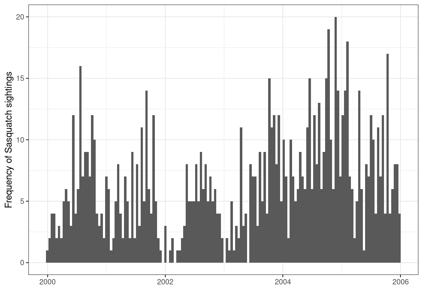
ggplot(sasquatch) +
  geom_sf(alpha = 0.3) +
  coord_sf() +
  geom_sf(data = us, fill = NA) +
  theme_classic()
Coordinate system already present. Adding new coordinate system, which will
replace the existing one.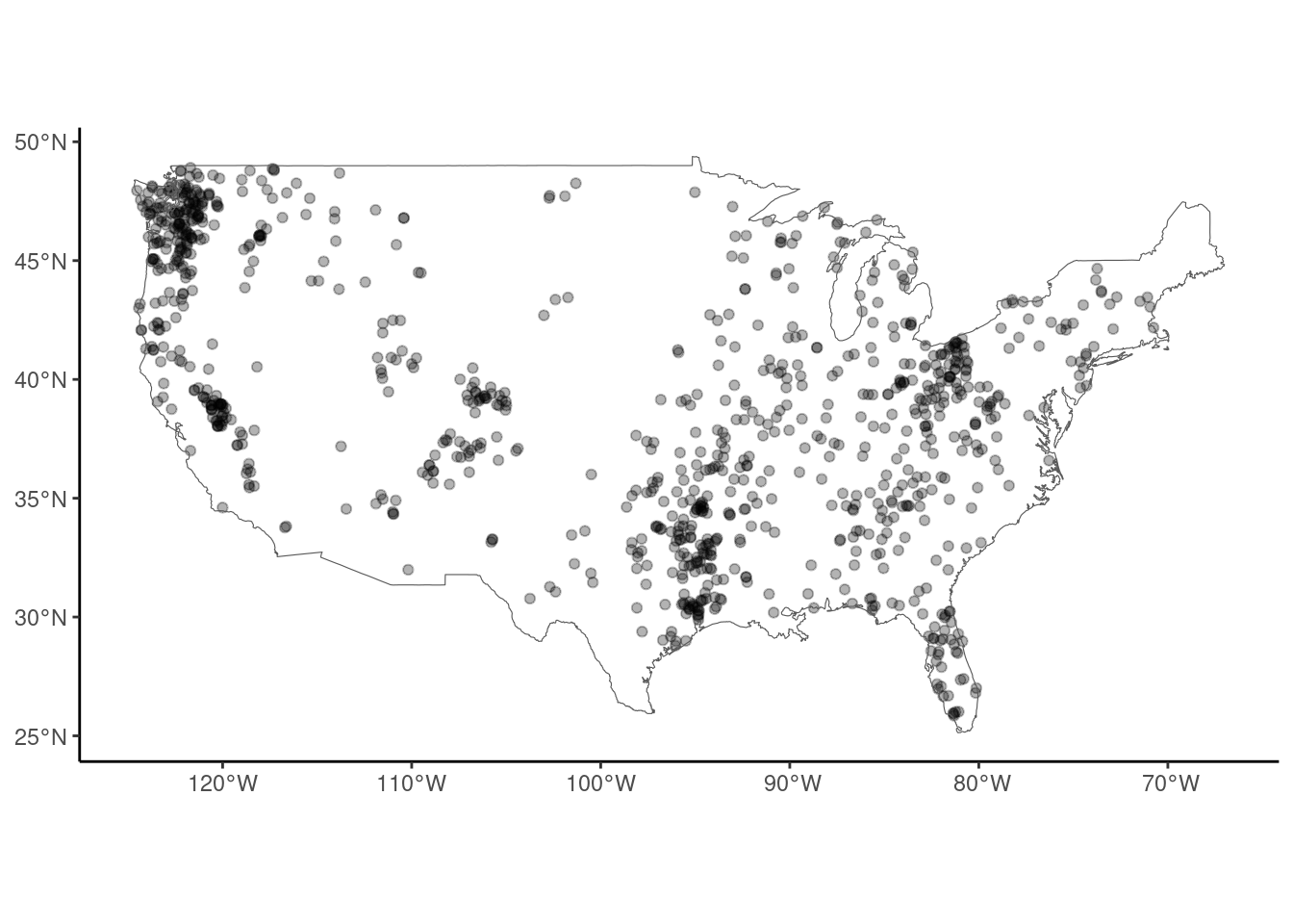
nz_earthquakesGeoNet Quake Search catalogues New Zealand earthquake occurrence; some of these data have been and packaged in stelfi as nz_earthquakes. In this chapter a Hawkes process is fitted to these data.
data("nz_earthquakes", package = "stelfi")
nz_earthquakes
Simple feature collection with 3824 features and 3 fields
Geometry type: POINT
Dimension: XY
Bounding box: xmin: 169.83 ymin: -44.86892 xmax: 175.6328 ymax: -41.8628
Geodetic CRS: +proj=longlat +datum=WGS84 +no_defs +ellps=WGS84 +towgs84=0,0,0
First 10 features:
origintime magnitude depth geometry
1 2014-12-24 07:46:00 3.208996 13.671875 POINT (172.7133 -43.57944)
2 2014-12-24 06:43:00 4.109075 5.820312 POINT (172.7204 -43.55752)
3 2014-12-14 08:53:00 3.240377 5.058594 POINT (172.3641 -43.62563)
4 2014-12-12 13:37:00 4.459034 9.394531 POINT (172.368 -43.63492)
5 2014-11-20 08:24:00 3.116447 10.039062 POINT (172.7836 -43.42493)
6 2014-11-18 14:19:00 3.158710 11.269531 POINT (172.7936 -43.4897)
7 2014-11-02 06:45:00 3.708697 14.960938 POINT (170.2523 -44.48656)
8 2014-10-11 22:32:00 3.456145 39.804688 POINT (173.1383 -42.67562)
9 2014-10-01 20:58:00 3.106894 11.386719 POINT (172.6879 -43.49002)
10 2014-09-30 15:29:00 3.911931 9.335938 POINT (172.1428 -43.25048)ggplot(nz_earthquakes, aes(x = origintime)) + geom_histogram(bins = 100) +
ylab("Frequency of earthquakes") + xlab("") +
theme_bw()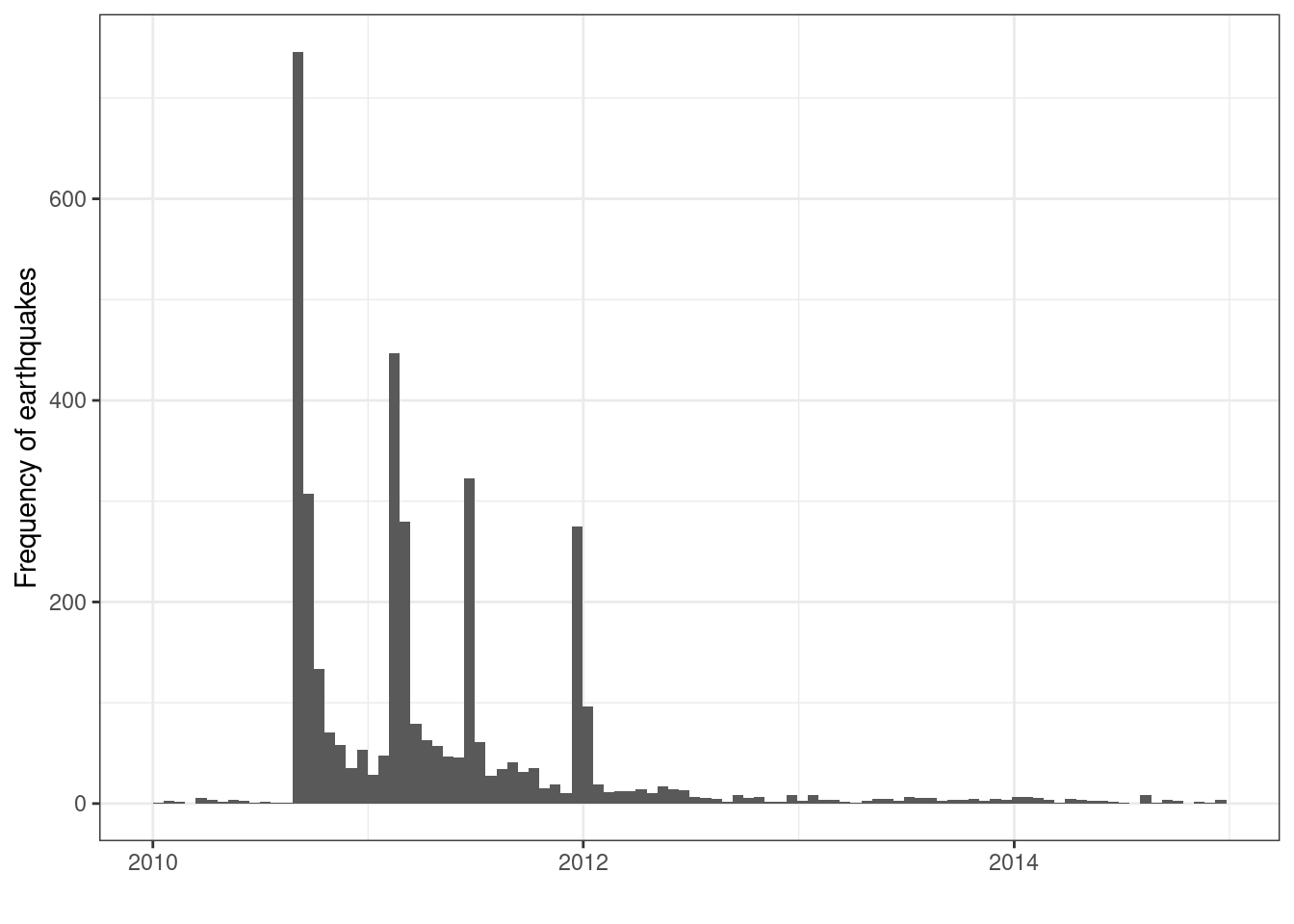
ggplot(nz_earthquakes) +
  geom_sf(alpha = 0.1) +
  coord_sf() +
  geom_sf(data = nz, fill = NA) +
  theme_classic()
Coordinate system already present. Adding new coordinate system, which will
replace the existing one.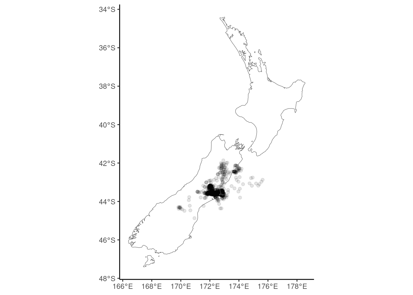
nz_murdersThe Homicide Report documents homicides in New Zealand. The nz_murders dataset contains summary information about the documented cases. In this chapter a spatiotemporal self-exciting model is fitted to these data.
data("nz_murders", package = "stelfi")
nz_murders
Simple feature collection with 967 features and 11 fields
Geometry type: POINT
Dimension: XY
Bounding box: xmin: 167.9161 ymin: -46.96127 xmax: 178.3955 ymax: -34.54022
Geodetic CRS: +proj=longlat +datum=WGS84 +no_defs +ellps=WGS84 +towgs84=0,0,0
First 10 features:
sex age date year cause killer
1 Male 41 Jan 5 2004 stabbing friend
2 Male 46 Jan 8 2004 pick axe wounds friend
3 Male 0 Jan 15 2004 asphyxiation (suffocation) mother
4 Female 46 Feb 1 2004 blunt force trauma partner
5 Male 10 Feb 2 2004 stabbing father
6 Female 2 Feb 2 2004 stabbing father
7 Male 36 Feb 4 2004 stabbing partners ex-partner
8 Male 20 Feb 8 2004 car crash friend
9 Male 29 Feb 8 2004 blunt force trauma strangers
10 Female 32 Feb 15 2004 blunt force trauma husband
name full_date month cause_cat region
1 Donald Linwood 2004-01-05 January Violent weapon Canterbury
2 James Weeks 2004-01-08 January Violent weapon Canterbury
3 Gabriel Harrison-Taylor 2004-01-15 January Asphyxia Auckland
4 Odette Lloyd-Rangiuia 2004-02-01 February Blunt force trauma Canterbury
5 Te Hau OCarroll 2004-02-02 February Violent weapon Wellington
6 Ngamata OCarroll 2004-02-02 February Violent weapon Wellington
7 Darryn McRobert 2004-02-04 February Violent weapon Canterbury
8 Peretiso Sauni 2004-02-08 February Car crash Auckland
9 Shannon McComb 2004-02-08 February Blunt force trauma Canterbury
10 Asolelei Sameulu 2004-02-15 February Blunt force trauma Auckland
geometry
1 POINT (171.6442 -43.63394)
2 POINT (172.1305 -43.28563)
3 POINT (174.8498 -36.92575)
4 POINT (172.6327 -43.55006)
5 POINT (175.1195 -40.73297)
6 POINT (175.1193 -40.73273)
7 POINT (172.5172 -43.53866)
8 POINT (174.7335 -36.89708)
9 POINT (172.6429 -43.54363)
10 POINT (174.6274 -36.90353)ggplot(nz_murders, aes(x = full_date)) + geom_histogram(bins = 100) +
ylab("Frequency of murders") + xlab("") +
theme_bw()Warning: Removed 8 rows containing non-finite outside the scale range
(`stat_bin()`).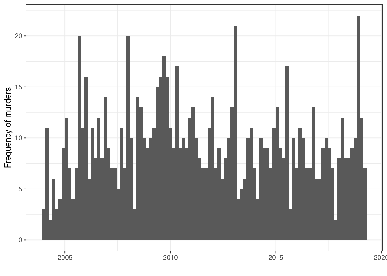
iraq_terrorismThe Global Terrorism Database (GTD) documents information on terrorism events worldwide; some of these data have been and packaged in stelfi as iraq_terrorism.
data("iraq_terrorism", package = "stelfi")
iraq_terrorism
Simple feature collection with 4208 features and 16 fields
Geometry type: POINT
Dimension: XY
Bounding box: xmin: 38.92288 ymin: 30.51005 xmax: 47.7781 ymax: 36.92948
Geodetic CRS: +proj=longlat +datum=WGS84 +no_defs +ellps=WGS84 +towgs84=0,0,0
First 10 features:
iyear imonth iday country success nkill specificity
18055 2013 4 18 Iraq TRUE 28 1
18109 2013 4 20 Iraq TRUE 0 1
18110 2013 4 20 Iraq TRUE 0 1
18111 2013 4 20 Iraq TRUE 0 1
18864 2013 5 16 Iraq TRUE 3 1
18865 2013 5 16 Iraq TRUE 3 1
18866 2013 5 16 Iraq TRUE 2 1
18867 2013 5 16 Iraq TRUE 3 1
19161 2013 5 27 Iraq TRUE 6 1
19166 2013 5 27 Iraq TRUE 1 1
gname x_coord y_coord z_coord
18055 Islamic State of Iraq and the Levant (ISIL) 0.5974251 0.5844656 0.5490748
18109 Islamic State of Iraq and the Levant (ISIL) 0.5997164 0.5864987 0.5443892
18110 Islamic State of Iraq and the Levant (ISIL) 0.5992751 0.5859289 0.5454876
18111 Islamic State of Iraq and the Levant (ISIL) 0.5959873 0.5733453 0.5622049
18864 Islamic State of Iraq and the Levant (ISIL) 0.5974251 0.5844656 0.5490748
18865 Islamic State of Iraq and the Levant (ISIL) 0.5974251 0.5844656 0.5490748
18866 Islamic State of Iraq and the Levant (ISIL) 0.5974251 0.5844656 0.5490748
18867 Islamic State of Iraq and the Levant (ISIL) 0.5876310 0.5507342 0.5927745
19161 Islamic State of Iraq and the Levant (ISIL) 0.5974251 0.5844656 0.5490748
19166 Islamic State of Iraq and the Levant (ISIL) 0.5974251 0.5844656 0.5490748
popdensity luminosity tt utm_x utm_y
18055 0.4065874 1.0924644 -0.3210921 333098.1 4007920.00
18109 -0.3479151 0.2298066 -0.2726546 407264.8 5332968.87
18110 -0.3479432 0.9717434 -0.3210921 401682.9 5252649.56
18111 -0.3783331 1.0521158 -0.3210921 405272.2 5344797.97
18864 0.4065874 1.0924644 -0.3210921 595450.3 4078540.46
18865 0.4065874 1.0924644 -0.3210921 595450.3 4078540.46
18866 0.4065874 1.0924644 -0.3210921 723492.7 45579.28
18867 -0.3665068 1.0924644 -0.3210921 815931.5 435892.29
19161 0.4065874 1.0924644 -0.3210921 252226.3 3703963.04
19166 0.4065874 1.0924644 -0.3210921 756886.0 4023175.15
geometry
18055 POINT (44.37177 33.30357)
18109 POINT (44.3616 32.98293)
18110 POINT (44.35484 33.05799)
18111 POINT (43.89071 34.20842)
18864 POINT (44.37177 33.30357)
18865 POINT (44.37177 33.30357)
18866 POINT (44.37177 33.30357)
18867 POINT (43.14357 36.35415)
19161 POINT (44.37177 33.30357)
19166 POINT (44.37177 33.30357)iraq_terrorism %>%
mutate(date = paste(iday, imonth, iyear, sep = "/")) %>%
mutate(date = as.Date(date, "%d/%m/%Y")) %>%
ggplot(., aes(x = date)) + geom_histogram(bins = 150) +
ylab("Frequency of attacks") + xlab("") +
theme_bw()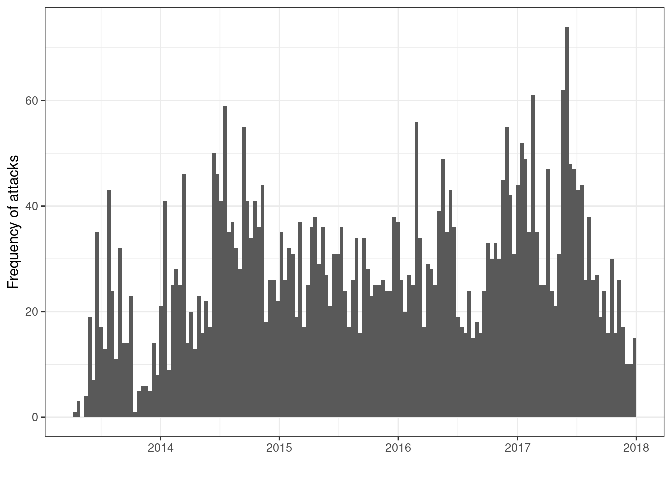
ggplot(iraq_terrorism) +
  geom_sf(alpha = 0.3) +
  coord_sf() +
  geom_sf(data = iraq, fill = NA) +
  theme_classic()
Coordinate system already present. Adding new coordinate system, which will
replace the existing one.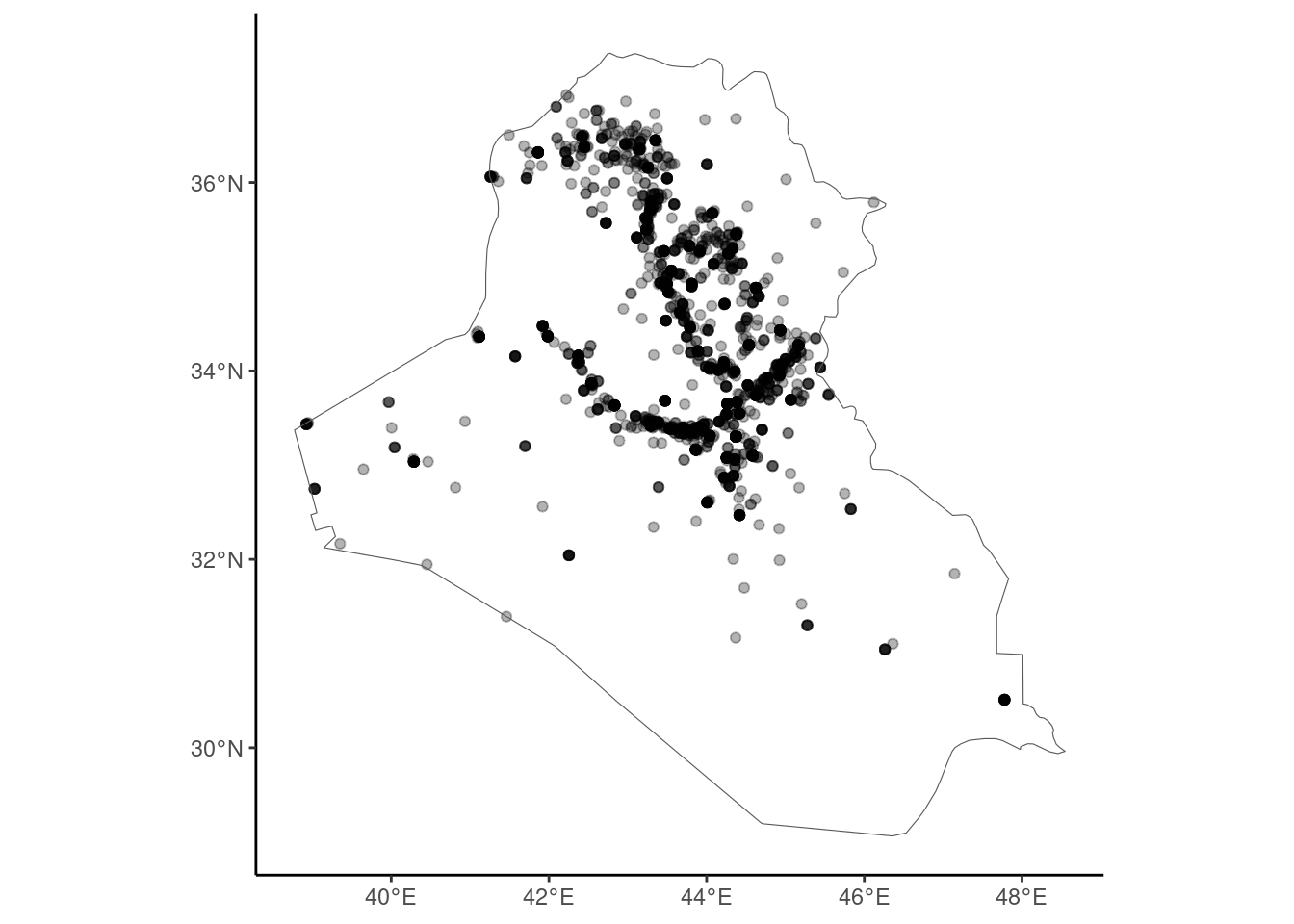
xytIn this chapter a log-Gaussian Cox process is fitted to these data and in this chapter a spatiotemporal selfexciting model is fitted.
data("xyt", package = "stelfi")
xyt_sf <- sf::st_as_sf(xyt)
xyt_sf
Simple feature collection with 654 features and 1 field
Geometry type: GEOMETRY
Dimension: XY
Bounding box: xmin: 0 ymin: -2.974928 xmax: 12.56637 ymax: 2.974928
CRS: NA
First 10 features:
label geom
1 window POLYGON ((10.77117 -2.78183...
2 point POINT (6.8074 -2.034423)
3 point POINT (7.558362 -2.193865)
4 point POINT (8.085083 -2.080938)
5 point POINT (8.121308 -2.522357)
6 point POINT (8.362448 -2.303117)
7 point POINT (9.000749 -2.955328)
8 point POINT (9.147803 -2.243146)
9 point POINT (9.261744 -2.408326)
10 point POINT (8.532312 -2.48986)ggplot(xyt_sf) + geom_sf(fill = NA) +
theme_void()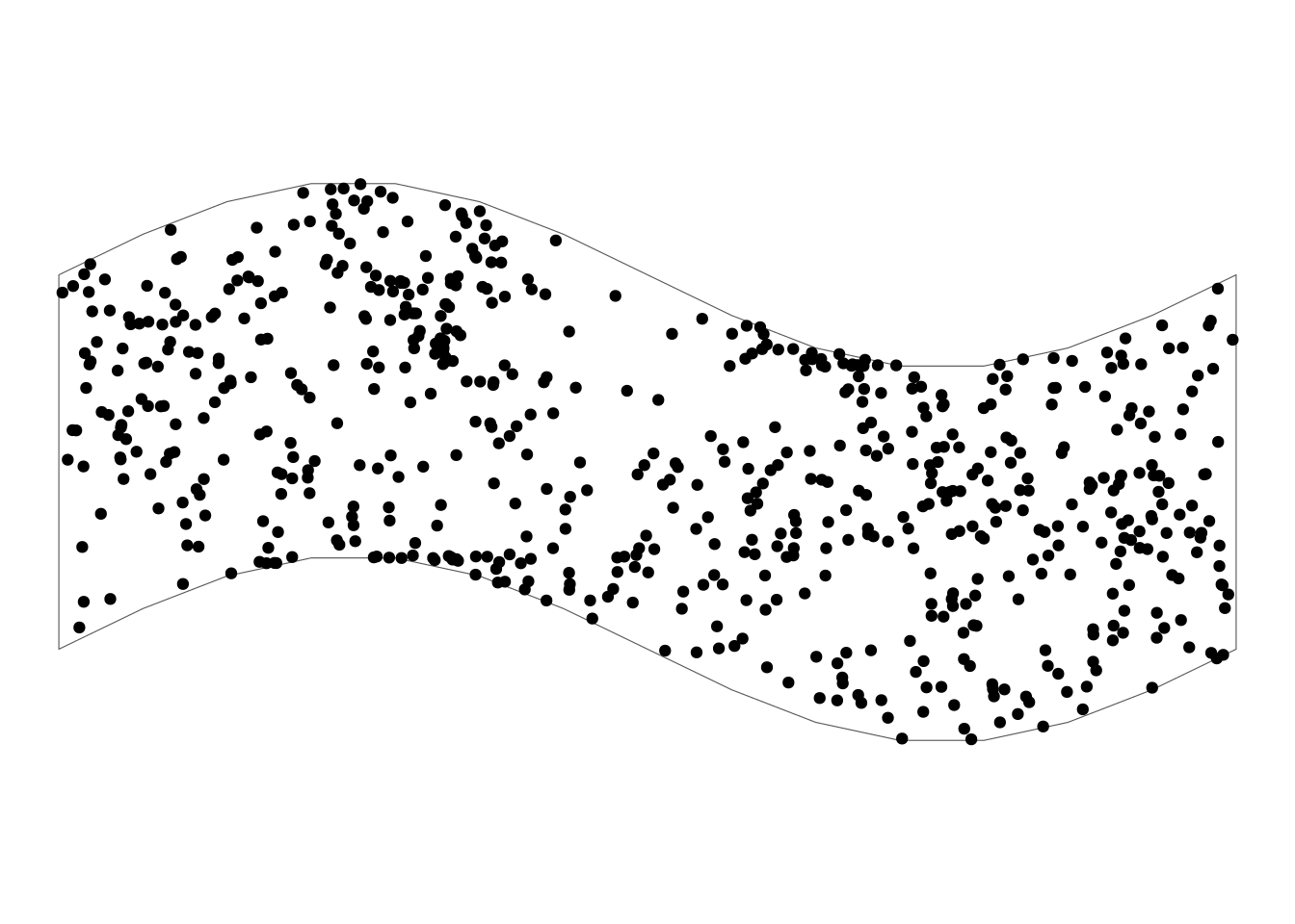
markedIn this chapter a marked log-Gaussian Cox process is fitted to these data.
data(marked, package = "stelfi")
marked_sf <- sf::st_as_sf(x = marked,
                        coords = c("x", "y"))
marked_sf
Simple feature collection with 159 features and 3 fields
Geometry type: POINT
Dimension: XY
Bounding box: xmin: 0.006606752 ymin: 0.006502493 xmax: 2.985087 ymax: 2.938558
CRS: NA
First 10 features:
m1 m2 m3 geometry
1 10.008609 0 9.616468 POINT (0.08935799 0.5756269)
2 8.730592 0 6.918024 POINT (2.177973 2.90455)
3 11.330677 0 16.798212 POINT (2.250791 1.024792)
4 11.338656 0 8.073566 POINT (2.033398 1.038773)
5 9.395725 0 9.977866 POINT (2.777002 0.4685442)
6 10.331965 0 10.615245 POINT (0.5988652 2.422233)
7 10.069787 0 11.268171 POINT (1.541071 0.9307671)
8 9.717775 0 13.306125 POINT (2.615062 1.064561)
9 10.071326 0 18.300715 POINT (0.3882139 2.146845)
10 10.147740 0 16.751740 POINT (1.501552 1.64466)domain <- list(3 * cbind(c(0, 1, 1, 0, 0), c(0, 0, 1, 1, 0))) %>%
sf::st_polygon() %>% sf::st_sfc() %>% sf::st_sf(geometry = .)
ggplot(marked_sf, aes(col = m1)) +
geom_sf() + labs(color = "Mark") +
scale_color_continuous(type = "viridis") +
geom_sf(data = domain, fill = NA, inherit.aes = FALSE) +
theme_void()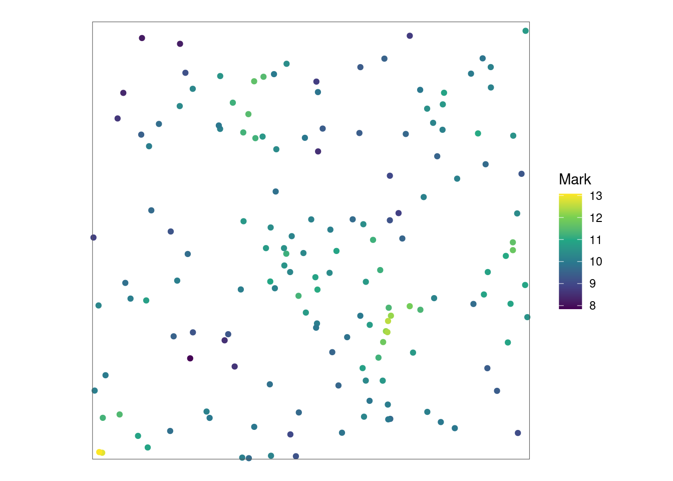
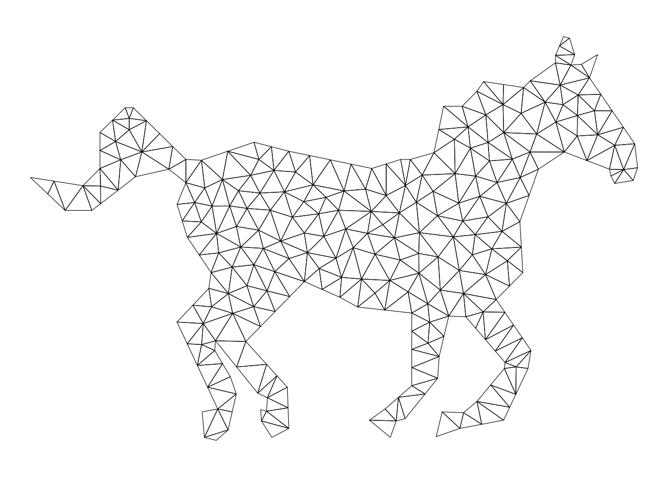
horse_meshIn this chapter we illustrate different geometric metrics of this triangulation.
data("horse_mesh", package = "stelfi")
horse_mesh_sf <- stelfi::mesh_2_sf(horse_mesh)
horse_mesh_sf
Simple feature collection with 396 features and 4 fields
Geometry type: POLYGON
Dimension: XY
Bounding box: xmin: -17.96875 ymin: -11.78261 xmax: 17.26563 ymax: 11.65217
CRS: NA
First 10 features:
V1 V2 V3 ID geometry
1 172 30 186 1 POLYGON ((8.441837 -2.16176...
2 28 188 162 2 POLYGON ((10.43359 0.913043...
3 168 186 42 3 POLYGON ((5.818232 -3.05894...
4 117 57 63 4 POLYGON ((-3.660156 -8.0326...
5 270 253 121 5 POLYGON ((-8.43636 2.023352...
6 92 144 169 6 POLYGON ((-8.042969 4.47826...
7 175 137 240 7 POLYGON ((5.689521 -1.13385...
8 182 148 111 8 POLYGON ((10.50244 7.199319...
9 253 169 121 9 POLYGON ((-7.850425 2.87106...
10 14 15 116 10 POLYGON ((13.3125 11.56522,...ggplot(horse_mesh_sf) + geom_sf(fill = NA, col = "black") +
theme_void()