4 Multivariate Hawkes
A multivariate Hawkes process allows for between- and within-stream self-excitement. In stelfi the conditional intensity for the \(j^{th}\) (\(j = 1, ..., N\)) stream is given by
\[\lambda(t)^{j*} = \mu_j + \Sigma_{k = 1}^N\Sigma_{i:\tau_i<t} \alpha_{jk} e^{(-\beta_j * (t-\tau_i))},\] where \(j, k \in (1, ..., N)\). Here, \(\alpha_{jk}\) is the excitement caused by the \(k^{th}\) stream on the \(j^{th}\). Therefore, \(\boldsymbol{\alpha}\) is an \(N \times N\) matrix where the diagonals represent the within-stream excitement and the off-diagonals represent the excitement between streams.
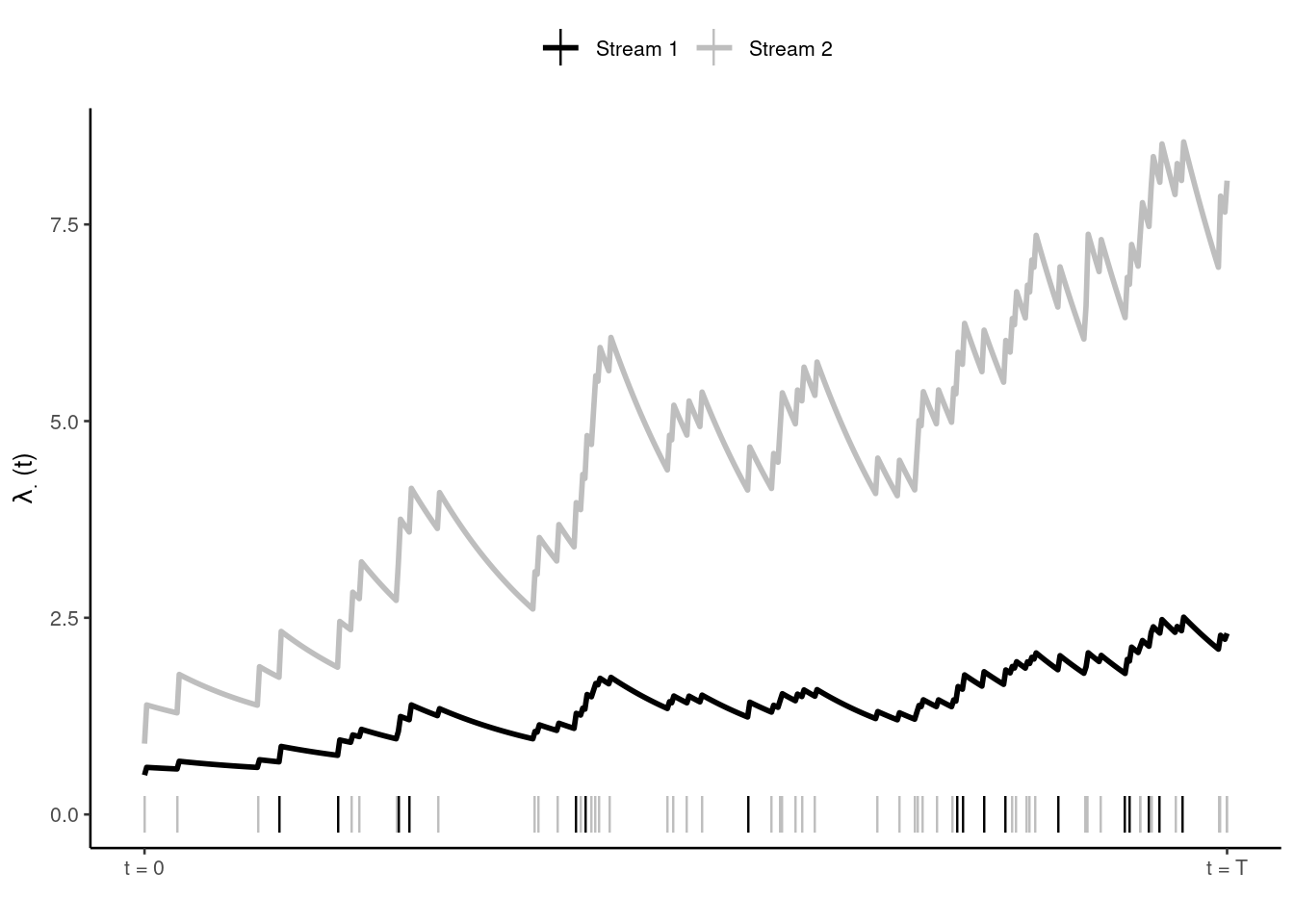
Plotted below are the conditional intensities (\(\lambda_{.}(t), t \in [0,T]\)) of a bivariate Hawkes process with \(\mu = (0.5, 0.9)\), \(\boldsymbol{\alpha}\) = \(\begin{bmatrix}0.2&0.1 \\0.6&0.5 \\\end{bmatrix}\), and \(\beta = (0.7, 0.9)\). Observed events (n = 33) are shown by the vertical dashes along the x-axis. The intensity of any stream increases immediately after any event occurs (i.e., irrespective of stream) and decays exponentially over time if no event is observed for some period. Typically, herem a jump in intensity due to the occurence of an event in the same stream is called self-excitation (diagonal elements of \(\boldsymbol{\alpha}\)) and a jump in intensity due to the occurence of an event in a different stream is called cross-excitation (off-diagonal elements of \(\boldsymbol{\alpha}\)).

4.1 A simulated example
Simulating data from the hawkes package Zaatour (2014) with \(\mu = (0.5, 0.9)\), \(\boldsymbol{\alpha}\) = \(\begin{bmatrix}0.2&0.1 \\0.6&0.5 \\\end{bmatrix}\), and \(\beta = (0.7, 0.9)\) over the time period \(t\in [0,50)\).
mu <- c(0.5, 0.9)
alpha <- matrix(c(0.2, 0.1 ,0.6, 0.5), byrow = TRUE, nrow = 2)
beta <- c(0.7, 0.9)
set.seed(1)
sim <- hawkes::simulateHawkes(mu, alpha, beta, 500)
To fit the model in stelfi the fit_mhawkes() function is used with the arguments times (a numeric vector of event times), stream (a character vector specifying the stream ID of each observation in times), and a lit of starting value for the parameters (parameters).
## reformat data for fitting
data <- data.frame(times = unlist(sim), stream =  rep(c("Stream 1", "Stream 2"),
                                                      times = sapply(sim, length)))
data <- data[order(data$times),]
## list of starting values
sv <- list(mu =  mu,alpha = alpha, beta = beta)
fit <- stelfi::fit_mhawkes(times = data$times, stream = data$stream, parameters = sv)


get_coefs(fit)
Estimate Std. Error
mu 0.7499955 0.10506748
mu 0.9852693 0.18009767
alpha 0.1617181 0.07753682
alpha 0.5438258 0.20395221
alpha 0.1225411 0.02940381
alpha 0.6091406 0.08140212
beta 1.0979208 0.63608232
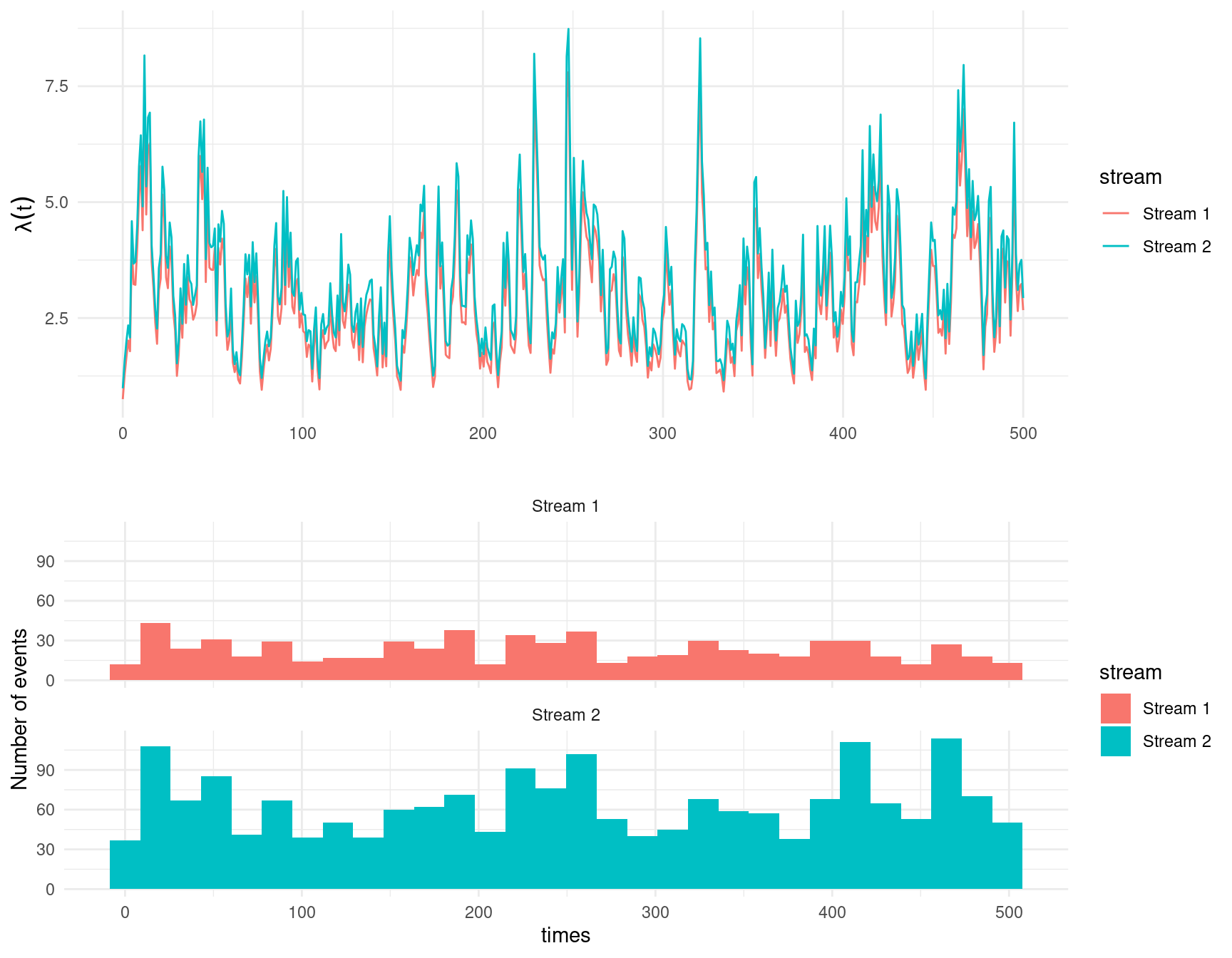
beta 1.0725560 0.17178757The fitted model is plotted using show_multivariate_hawkes() (default type = "fitted")
show_multivariate_hawkes(fit, type = "both")