Loading required package: stelfi| mark | jump |
|---|---|
| 1 | 0.4 |
| 2 | 0.8 |
| 3 | 1.2 |
| 4 | 1.6 |
The conditional intensity function for the marked Hawkes model implemented in stelfi is given by
\[\lambda(t; m(t)) = \mu + \alpha \Sigma_{i:\tau_i<t}m(\tau_i)\text{exp}(-\beta * (t-\tau_i)) \] where \(\mu\) is the background rate of the process and \(m(t)\) is the temporal mark. The only difference to Equation 2.1 is now that each event has an associated mark \(m(\tau_i)\) that scales the jump sizes (\(\alpha\)) of the self-exciting component of \(\lambda(.)\).
Below data are simulated using the emhawkes package (Lee 2023) where the marks (a vector that scale the jump sizes, starting at 0) are integer values \(\in [1,4]\) for \(t > 0\) and \(0\) for \(t = 0\) (see Section 3.2 for how to simulate using stelfi). The parameter values of the conditional intensity are \(\mu = 1.3\), \(\alpha = 0.4\), and \(\beta = 1.5\). The jump sizes for the possible mark values are shown below.
Loading required package: stelfi| mark | jump |
|---|---|
| 1 | 0.4 |
| 2 | 0.8 |
| 3 | 1.2 |
| 4 | 1.6 |
require(emhawkes)
mu <- 1.3; alpha <- 0.4; beta <-  1.5
fn_mark <- function( ...){
    sample(1:4, 1)
}
h1 <- new("hspec", mu = mu, alpha = alpha, beta = beta,
          rmark = fn_mark)
set.seed(123)
res <- hsim(h1, size = 100)
To fit the model in stelfi the fit_hawkes() function is used and the additional optional argument marks supplied.
sv <- c(mu = 1.3, alpha = 0.4, beta = 1.5)
fit <- fit_hawkes(times = res$arrival, parameters = sv, marks = res$mark)
get_coefs(fit)
Estimate Std. Error
mu 1.1741551 0.25195698
alpha 0.1008830 0.06935281
beta 0.8849185 0.50179668Note the estimated coefficient \(\alpha\) from stelfi equates to \(\frac{\alpha}{\text{mark}}\) from emhawkes.
## benchmark emhawkes
emhawkes::hfit(h1, inter_arrival = res$inter_arrival, mark = res$mark) |>
  summary()
--------------------------------------------
Maximum Likelihood estimation
BFGS maximization, 43 iterations
Return code 0: successful convergence
Log-Likelihood: -51.99802
3 free parameters
Estimates:
Estimate Std. error t value Pr(> t)
mu1 1.1106 0.2888 3.845 0.00012 ***
alpha1 0.2787 0.1903 1.464 0.14309
beta1 0.9277 0.5693 1.629 0.10321
---
Signif. codes: 0 '***' 0.001 '**' 0.01 '*' 0.05 '.' 0.1 ' ' 1
--------------------------------------------The fitted model and diagnostic plots are plotted using show_hawkes() and show_hawkes_GOF().
show_hawkes(fit)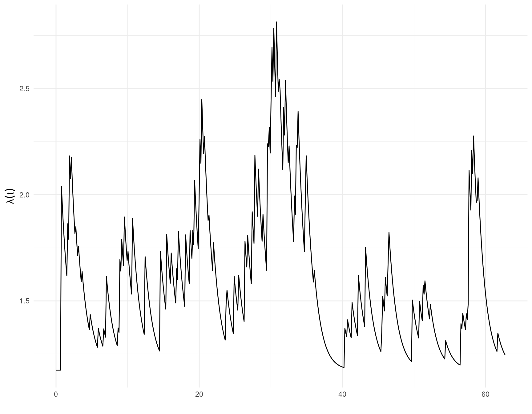
show_hawkes_GOF(fit)
    Exact one-sample Kolmogorov-Smirnov test

data:  interarrivals
D = 0.09164, p-value = 0.355
alternative hypothesis: two-sided


    Box-Ljung test

data:  interarrivals
X-squared = 0.38285, df = 1, p-value = 0.5361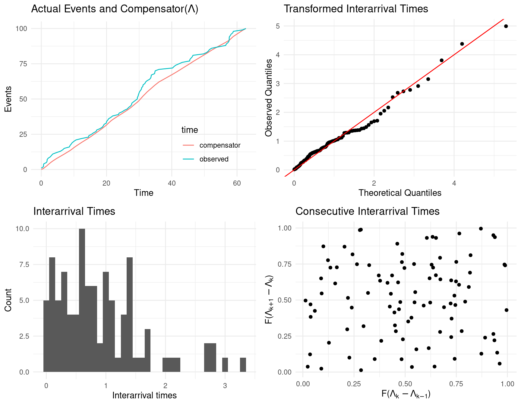
TODO
Below the negative log-likelihood of a univariate marked Hawkes process used by stelfi is written using R/RTMB (Kristensen 2024) syntax. The function below returns the negative log-likelihood of a univariate marked Hawkes process, RTMB is used to automatically calculate the gradient and then the function is minimised via nlminb(). See here for and overview of RTMB. This section is for demonstration only, feel free to modify the function as desired. Note that this can be used to fit an unmarked model by setting the vector of marks to be \(\boldsymbol{1}\).
library(RTMB)
univariate_marked_hawkes <- function(params){
    getAll(data, params)
    mu <- exp(log_mu)
    beta <- exp(log_beta)
    alpha <- exp(logit_abratio) / (1 + exp(logit_abratio)) * (beta/mean(marks))
    n <- length(times)
    last <- times[n]
    nll <- 0
    A <- advector(numeric(n))
    for(i in 2:n){
        A[i] <- sum(exp(-beta * (times[i] - times[i - 1])) * (marks[i - 1] + A[i - 1]))
    }
    term_3vec <- log(mu + alpha * A)
    nll <- (mu * last) + ((alpha/beta) * (sum(marks) - marks[n] - A[n])) - sum(term_3vec)
    ADREPORT(mu)
    ADREPORT(alpha)
    ADREPORT(beta)
    return(nll)
}

data <- list(times = res$arrival, marks = res$mark)
params <- list(log_mu = log(1.3), logit_abratio = 0.6, log_beta = log(1.5))
obj <- MakeADFun(univariate_marked_hawkes, params, silent = TRUE)
opt <- nlminb(obj$par, obj$fn, obj$gr)
summary(sdreport(obj), "report")
Estimate Std. Error
mu 1.1742764 0.25196080
alpha 0.1008268 0.06934413
beta 0.8846088 0.50173890