5 Lyric Sentiments
require(sentimentr)
require(taylor)
require(ggrepel)
## taylor_album_songs from taylor package
lyrics_df <- taylor_album_songs %>%
unnest(lyrics) %>%
select(album_name, track_name, track_number, line, lyric, element)
lyrics_df$row_id <- 1:nrow(lyrics_df)
sentences_with_id <- get_sentences(lyrics_df$lyric, lyrics_df$row_id) # this processes
## each line as its own sentence as it's using the row_id.
sentiment_with_id <- sentiment(sentences_with_id)
sentiment_summary <- sentiment_with_id %>%
group_by(element_id) %>%
summarise(
avg_sentiment = mean(sentiment, na.rm = TRUE),
word_count = sum(word_count)
)
## Join
lyrics_sentiment <- lyrics_df %>%
left_join(sentiment_summary, by = c("row_id" = "element_id"))
## Aggregate by song to get net sentiment score
song_sentiment_scores_sentimentr <- lyrics_sentiment %>%
group_by(track_number, track_name, album_name) %>%
summarize(
sum_sentiment = sum(avg_sentiment),
total_sentiment_words = n(),
avg_sentiment = sum(avg_sentiment) / n(),
.groups = "drop"
)albumOrder <- c("Taylor Swift", "Fearless (Taylor's Version)",
"Speak Now (Taylor's Version)", "Red (Taylor's Version)",
"1989 (Taylor's Version)", "Reputation", "Lover",
"folklore", "evermore", "Midnights",
"THE TORTURED POETS DEPARTMENT")
lyrics_sentiment <- lyrics_sentiment %>%
mutate(album_name = factor(album_name, levels = albumOrder))
lyrics_sentiment <- lyrics_sentiment %>%
filter(!is.na(album_name))## Plot the net sentiment scores
ggplot(lyrics_sentiment, aes(x = track_number, y = avg_sentiment, fill = album_name)) +
geom_col(show.legend = FALSE) +
facet_wrap(~album_name, ncol = 3, scales = "free") +
scale_fill_manual(values = colorPaletteAlbums) +
theme_minimal() +
labs(
title = "The emotional spectrum across Taylor Swift's discography",
x = "Track Number",
y = "Net Sentiment (Positive - Negative Words)"
) +
theme(plot.title = element_text(hjust=0.5))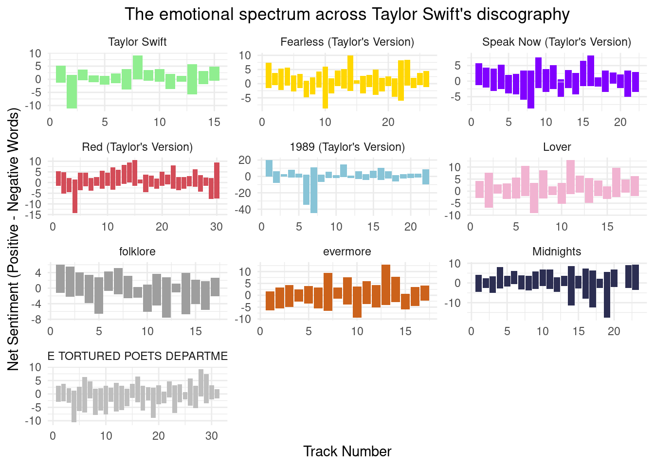
song_sentiment_scores_sentimentr <- lyrics_sentiment %>%
  group_by(track_number, track_name, album_name) %>%
  summarize(
    sum_sentiment = sum(avg_sentiment),
    total_sentiment_words = n(),
    avg_sentiment = sum(avg_sentiment) / n(),
    .groups = "drop"
  )

surpriseSongsDressColours <- surpriseSongsDressColours %>%
  mutate(DressColourGroup = case_when(
    DressName %in% c("Pink", "Flamingo pink") ~ "Reds",
    DressName %in% c("Blue", "Ocean blue") ~ "Blues",
    DressName %in% c("Yellow", "Sunset orange") ~ "Yellows",
    DressName %in% c("Cotton candy", "Grapefruit", "Popsicle") ~ "Colourful",
    DressName == "Blurple" ~ "Purples",
    DressName == "Green" ~ "Greens"
  ))

dress_song_sentiment_scores_sentimentr <- surpriseSongsDressColours %>%
  left_join(song_sentiment_scores_sentimentr, by = c("Song title" = "track_name")) %>%
  filter(!is.na(avg_sentiment))

dress_group_sentiments <- dress_song_sentiment_scores_sentimentr %>%
  group_by(DressColourGroup) %>%
  summarise(
    performance_weighted_sentiment = mean(avg_sentiment, na.rm = TRUE),
    n_performances = n(),
    .groups = 'drop'
  )
## recall the CA from before
colorSentimentScores$colourGroup <- colorGroups[colorSentimentScores$colour]
cols.df <- as.data.frame.matrix(table(colorSentimentScores$colourGroup, colorSentimentScores$meaning))
coa <- FactoMineR::CA(cols.df)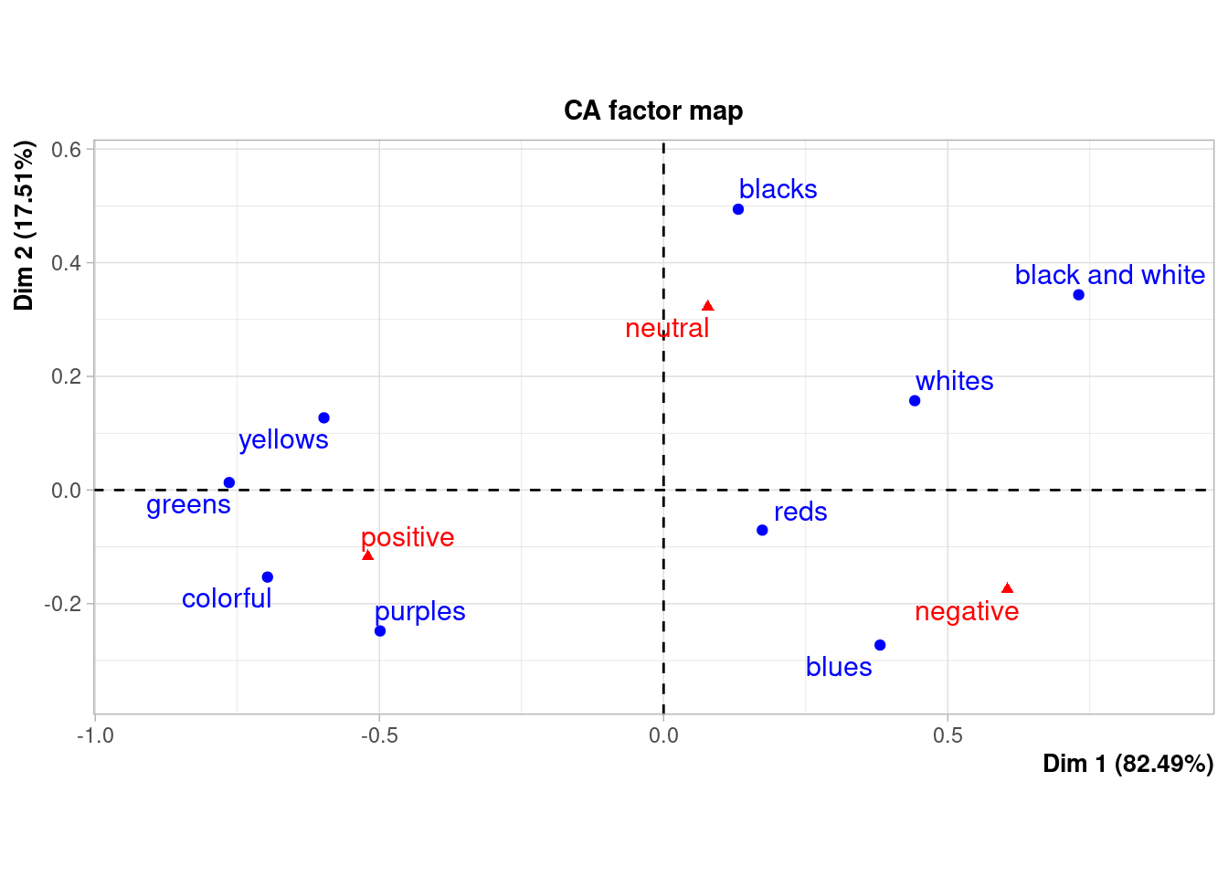
## here we flip so that dim 1 is "-ve --> +ve"
colour_coa_table <- coa$row$coord %*% diag(c(-1,1)) |>
as.data.frame() |>
rownames_to_column("colour_category") |>
select(colour_category, colour_sentiment = V1) |>
as_tibble()
colour_sentiments <- colour_coa_table %>%
mutate(
DressColourGroup = case_when(
colour_category == "blues" ~ "Blues",
colour_category == "colorful" ~ "Colourful",
colour_category == "greens" ~ "Greens",
colour_category == "purples" ~ "Purples",
colour_category == "reds" ~ "Reds",
colour_category == "yellows" ~ "Yellows",
TRUE ~ NA_character_
)
) %>%
filter(!is.na(DressColourGroup))
dress_group_sentiments <- dress_song_sentiment_scores_sentimentr %>%
group_by(DressColourGroup) %>%
summarise(
performance_weighted_sentiment = mean(avg_sentiment, na.rm = TRUE),
n_performances = n(),
.groups = 'drop'
)
combined_analysis <- dress_group_sentiments %>%
left_join(colour_sentiments, by = "DressColourGroup") %>%
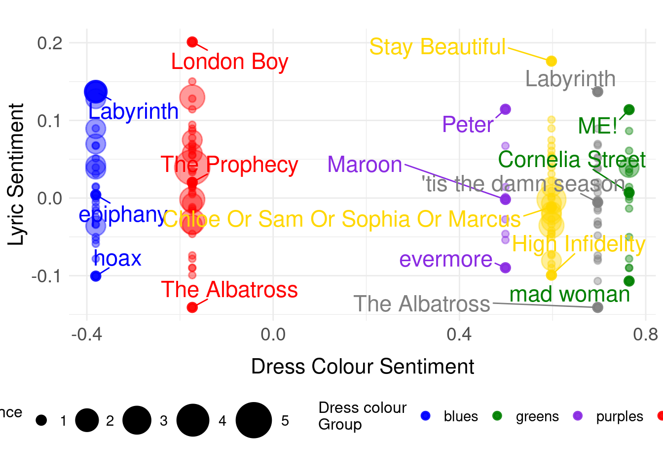
select(DressColourGroup, performance_weighted_sentiment, colour_sentiment, n_performances)Let’s plot.
song_performance_counts <- dress_song_sentiment_scores_sentimentr %>%
  group_by(`Song title`, DressColourGroup) %>%
  summarise(
    avg_sentiment = first(avg_sentiment),
    performance_count = n(),
    .groups = 'drop'
  )

plot_data <- song_performance_counts %>%
  left_join(colour_sentiments, by = "DressColourGroup") %>%
  filter(!is.na(colour_sentiment))


## Top songs (highest sentiment) for each color group
top_songs <- plot_data %>%
  group_by(DressColourGroup) %>%
  slice_max(avg_sentiment, n = 1, with_ties = FALSE) %>%
  ungroup()

## Bottom songs (lowest sentiment) for each color group
bottom_songs <- plot_data %>%
  group_by(DressColourGroup) %>%
  slice_min(avg_sentiment, n = 1, with_ties = FALSE) %>%
  ungroup()

## Medium songs (closest to median for each color group)
medium_songs <- plot_data %>%
  group_by(DressColourGroup) %>%
  mutate(
    median_sentiment = median(avg_sentiment, na.rm = TRUE),
    distance_from_median = abs(avg_sentiment - median_sentiment)
  ) %>%
  slice_min(distance_from_median, n = 1, with_ties = FALSE) %>%  # Closest to median per color (medium)
  ungroup()

highlight_songs <- bind_rows(
  top_songs,
  bottom_songs,
  medium_songs) %>%
  distinct(`Song title`, DressColourGroup, .keep_all = TRUE)


ggplot(plot_data, aes(x = colour_sentiment, y = avg_sentiment)) +
   geom_point(aes(size = performance_count, colour = tolower(DressColourGroup)),
             alpha = 0.4, stroke = 0.8) +
    geom_point(data = highlight_songs,
             aes(size = performance_count, colour = tolower(DressColourGroup)),
             alpha = 0.9, stroke = 1.5) +
    geom_text_repel(data = highlight_songs,
                  aes(label = `Song title`, colour = tolower(DressColourGroup)),
                  size = 6,
                  max.overlaps = Inf,
                  box.padding = 0.5,
                  point.padding = 0.3,
                  min.segment.length = 0.1,
                  show.legend = FALSE) +
  scale_size_continuous(name = "Performance\nCount",
                        range = c(2, 12),
                        breaks = c(1, 2, 3, 4, 5),
                        guide = guide_legend(override.aes = list(alpha = 1))) +
  scale_colour_manual(values = colorPaletteGroups,
                      name = "Dress colour\nGroup") +
    labs(title = "",
       subtitle = "",
       x = "Dress Colour Sentiment",
       y = "Lyric Sentiment",
       caption = "") +
  theme_minimal() +
  theme(
    plot.title = element_blank(),
    axis.title.x = element_text(size = 16,
                                margin = margin(t = 10)),
    axis.title.y = element_text(size = 16),
    axis.text = element_text(size = 14),
    legend.title = element_text(size = 12),
    legend.text = element_text(size = 11),
    legend.position = "bottom",
    legend.box = "horizontal"
  )
What about group-wise correlation?
## We only have 6 observations, not great, but let's go ahead anyway!
## Pearson's correlation
cor.test(combined_analysis$performance_weighted_sentiment,
                             combined_analysis$colour_sentiment)
    Pearson's product-moment correlation

data:  combined_analysis$performance_weighted_sentiment and combined_analysis$colour_sentiment
t = -5.4996, df = 4, p-value = 0.005329
alternative hypothesis: true correlation is not equal to 0
95 percent confidence interval:
 -0.9935629 -0.5403340
sample estimates:
       cor
-0.9397859
## Spearman's correlation
cor.test(combined_analysis$performance_weighted_sentiment,
combined_analysis$colour_sentiment,
method = "spearman")
    Spearman's rank correlation rho

data:  combined_analysis$performance_weighted_sentiment and combined_analysis$colour_sentiment
S = 54, p-value = 0.2972
alternative hypothesis: true rho is not equal to 0
sample estimates:
       rho
-0.5428571
## Spearman's correlation with 95% CIs
correlation::cor_test(data = combined_analysis,
x = "performance_weighted_sentiment",
y = "colour_sentiment",
method = "spearman")Parameter1 | Parameter2 | rho | 95% CI
-------------------------------------------------------------------------
performance_weighted_sentiment | colour_sentiment | -0.54 | [-0.94, 0.51]
Parameter1 | S | p
----------------------------------------------
performance_weighted_sentiment | 54.00 | 0.266
Observations: 6